Data Javascript Math

Harnessing X-Means Clustering and CIE2000 for Visually Striking Dominant Color Extraction

February 1st, 2024

Home Projects

Min K Max K Max Iterations

In the world of image processing and computer vision, extracting dominant colors from an image has become an increasingly important task. Whether you’re a data-driven designer looking to create visually appealing color palettes or a machine learning enthusiast exploring the intricacies of unsupervised learning, understanding how to accurately identify and quantify the most prominent colors in an image is a valuable skill. In this blog post, we’ll dive into the fascinating realm of dominant color extraction using the powerful combination of X-Means clustering and the CIE2000 color distance metric.

The X-Means clustering algorithm, an extension of the well-known K-Means algorithm, has gained significant attention in recent years due to its ability to automatically determine the optimal number of clusters in a dataset. By leveraging the principles of unsupervised machine learning, X-Means allows us to group similar colors together without requiring prior knowledge of the number of dominant colors present in an image. This adaptability makes X-Means a valuable tool for color quantization and palette generation tasks.

However, the effectiveness of any color clustering algorithm heavily relies on the choice of color distance metric. Traditional color spaces, such as RGB or HSV, often fail to accurately represent the perceptual differences between colors as perceived by the human eye. Developed by the International Commission on Illumination (CIE), CIE2000 takes into account the intricacies of human color perception, ensuring that the clustering process yields results that are visually meaningful and intuitive. By combining the power of X-Means clustering with the perceptual accuracy of CIE2000, we can unlock new possibilities in dominant color extraction, and image quantization.

Understanding X-Means Clustering🔗

To understand X-Means clustering we need to start with K-Means clustering. K-Means is a widely used unsupervised learning algorithm for clustering data points. It partitions a given dataset into a specified number of clusters (K) based on the similarity between data points. The algorithm follows these steps:

1. Initialization: Randomly select K data points as initial cluster centroids.
2. Assignment: Assign each data point to the nearest centroid based on a distance metric (e.g., Euclidean distance).
3. Update: Recalculate the centroids of each cluster by taking the mean of all data points assigned to that cluster.
4. Iteration: Repeat steps 2 and 3 until the centroids no longer change significantly or a maximum number of iterations is reached.

The goal of K-Means is to minimize the sum of squared distances between each data point and its assigned centroid, resulting in compact and well-separated clusters.

class KMeans {
    /**
     * A configurable implementation of the K-means clustering algorithm
     * 
     * 
     * @param {int} minK 
     * @param {Function} distanceMetric 
     * @param {object} options
     */

    constructor(minK, distanceMetric, options) {
        this.minK = minK;
        this.distanceMetric = distanceMetric;

        var options = options || {};
        this.distanceThreshold = options.distanceThreshold || 0.0; // minimum threshold of centroid changes to continue iterations
        this.maxIterations = options.maxIterations || Number.MAX_SAFE_INTEGER;
        this.meanFunc = options.meanFunc || this._arithmeticMean;
        this.kDTree = options.kDTree || false;
    }

    validateDataset(dataset) {
        if (!Array.isArray(dataset) || !dataset.length) {
            throw Error('dataset must be array');
        }

        if (dataset.length <= this.minK) {
            throw Error('dataset must have at least ' + this.minK + ' data points');
        }

        for (var i = 0; i < dataset.length; i++) {
            if (!Array.isArray(dataset[i])) {
                console.log(dataset[i]);
                throw Error('dataset points must be an array');
            }

            if (!dataset[i].length) {
                throw Error('dataset points must be a non-empty array');
            }
        }

        return true;
    }

    transform(dataset, options) {
        /**
         * Executes the k-means clustering algorithm against a dataset
         * with the given optional optimization parameters.  Parameters are
         * 
         * - validate (bool):  Indicates if the dataset should be validated
         * - kDTree (bool):  Indicates if a KD-tree should be used to find nearest centroids
         * 
         * @param {Array} dataset
         * @param {object} options
         */
        var options = options || {};
        options.kDTree = options.kDTree || this.kDTree;
        if (options.validate || true) {
            this.validateDataset(dataset);
        }

        let iterations = 0;
        let oldCentroids, labels, centroids;

        // Initialize centroids randomly
        if (options.useNaiveSharding || true) {
            centroids = this._getRandomCentroidsNaiveSharding(dataset);
        } else {
            centroids = this._getRandomCentroids(dataset);
        }

        // Run the main k-means algorithm
        while (!this._shouldStop(oldCentroids, centroids, iterations)) {
            // Save old centroids for convergence test.
            oldCentroids = [...centroids];
            iterations++;

            // Assign labels to each datapoint based on centroids
            labels = this._getLabels(dataset, centroids, options.kDTree);
            centroids = this._recalculateCentroids(dataset, labels);
        }

        const clusters = [];
        for (let i = 0; i < this.minK; i++) {
            clusters.push(labels[i]);
        }
        const results = {
            clusters: clusters,
            centroids: centroids,
            iterations: iterations,
            converged: iterations <= this.maxIterations,
        };
        return results;
    }

    _getLabels(dataSet, centroids, kDTree = true) {
        // prep data structure:
        const labels = {},
            centroidIndices = [];
        for (let c = 0; c < centroids.length; c++) {
            labels[c] = {
                points: [],
                centroid: centroids[c],
            };
            centroidIndices.push(c);
        }
        var tree;
        if (kDTree) {
            var centroidDimensions = centroids[0].map(function(v, i) {
                return i
            });
            tree = new KDTree(centroids, centroidIndices, centroidDimensions, this.distanceMetric);
        }
        // For each element in the dataset, choose the closest centroid. 
        // Make that centroid the element's label.
        for (let i = 0; i < dataSet.length; i++) {
            const a = dataSet[i];
            let closestCentroid, closestCentroidIndex
            if (kDTree) {
                var closestCentroids = tree.nearestNeighbor(a, 1);
                closestCentroid = closestCentroids[0],
                    closestCentroidIndex = closestCentroid.id;
            } else {
                let prevDistance;
                for (let j = 0; j < centroids.length; j++) {
                    let centroid = centroids[j];
                    if (j === 0) {
                        closestCentroid = centroid;
                        closestCentroidIndex = j;
                        prevDistance = this.distanceMetric(a, closestCentroid);
                    } else {
                        // get distance:
                        const distance = this.distanceMetric(a, centroid);
                        if (distance < prevDistance) {
                            prevDistance = distance;
                            closestCentroid = centroid;
                            closestCentroidIndex = j;
                        }
                    }
                }
            }
            // add point to centroid labels:
            labels[closestCentroidIndex].points.push(a);
        }
        return labels;
    }


    _compareDatasets(a, b) {
        for (let i = 0; i < a.length; i++) {
            if (a[i] !== b[i]) {
                return false;
            }
        }
        return true;
    }

    _getRandomCentroids(dataset) {
        // selects random points as centroids from the dataset
        const numSamples = dataset.length;
        const centroidsIndex = [];
        let index;
        while (centroidsIndex.length < this.minK) {
            index = this._randomBetween(0, numSamples);
            if (centroidsIndex.indexOf(index) === -1) {
                centroidsIndex.push(index);
            }
        }
        const centroids = [];
        for (let i = 0; i < centroidsIndex.length; i++) {
            const centroid = [...dataset[centroidsIndex[i]]];
            centroids.push(centroid);
        }
        return centroids;
    }

    _getRandomCentroidsNaiveSharding(dataset) {
        // implementation of a variation of naive sharding centroid initialization method
        // (not using sums or sorting, just dividing into k shards and calc mean)
        const numSamples = dataset.length;
        const step = Math.floor(numSamples / this.minK);
        const centroids = [];
        for (let i = 0; i < this.minK; i++) {
            const start = step * i;
            let end = step * (i + 1);
            if (i + 1 === this.minK) {
                end = numSamples;
            }
            centroids.push(this._calcMeanCentroid(dataset, start, end));
        }
        return centroids;
    }

    _calcMeanCentroid(dataSet, start, end) {
        const features = dataSet[0].length;
        const n = end - start;
        let mean = [];
        for (let i = 0; i < features; i++) {
            mean.push(0);
        }
        for (let i = start; i < end; i++) {
            for (let j = 0; j < features; j++) {
                mean[j] = mean[j] + dataSet[i][j] / n;
            }
        }
        return mean;
    }

    _shouldStop(oldCentroids, centroids, iterations) {
        if (iterations > this.maxIterations) {
            return true;
        }
        if (!oldCentroids || !oldCentroids.length) {
            return false;
        }

        if (oldCentroids.length === centroids.length) {
            let maxMovement = 0.0;
            for (let i = 0; i < centroids.length; i++) {
                const distance = this.distanceMetric(centroids[i], oldCentroids[i]);
                maxMovement = Math.max(maxMovement, distance);
            }

            if (maxMovement <= this.threshold) {
                return true;
            }

            let haveChanged = true;
            for (let i = 0; i < centroids.length; i++) {
                if (!this._compareDatasets(centroids[i], oldCentroids[i])) {
                    haveChanged = false;
                }
            }
            return haveChanged;
        }
        return false;
    }

    _recalculateCentroids(dataSet, labels) {
        // Each centroid is the arithmetic mean of the points that
        // have that centroid's label.  If no points have
        // a centroid's label, you should randomly re-initialize it.
        let newCentroid;
        const newCentroidList = [];
        for (const k in labels) {
            const centroidGroup = labels[k];
            if (centroidGroup.points.length > 0) {
                // find mean:
                newCentroid = this.meanFunc(centroidGroup.points);
            } else {
                // get new random centroid
                newCentroid = this._getRandomCentroids(dataSet, 1)[0];
            }
            newCentroidList.push(newCentroid);
        }
        return newCentroidList;
    }


    _arithmeticMean(dataset) {
        const totalPoints = dataset.length;
        const means = [];
        for (let j = 0; j < dataset[0].length; j++) {
            means.push(0);
        }
        for (let i = 0; i < dataset.length; i++) {
            const point = dataset[i];
            for (let j = 0; j < point.length; j++) {
                const val = point[j];
                means[j] = means[j] + val / totalPoints;
            }
        }
        return means;
    }

    _randomBetween(min, max) {
        return Math.floor(
            Math.random() * (max - min) + min
        );
    }
}

Despite its simplicity and effectiveness, K-Means has some limitations. One major drawback is that it requires the number of clusters (K) to be specified in advance. Determining the optimal value of K can be challenging, especially when dealing with complex datasets. If the chosen K does not align with the natural structure of the data, the resulting clusters may not be meaningful or representative. Moreover, K-Means is sensitive to the initial placement of centroids and may converge to suboptimal solutions. It can also struggle with clusters of different sizes, densities, or non-spherical shapes.

To address these limitations, an adaptive approach that can automatically determine the optimal number of clusters is desirable.

X-Means is an extension of the K-Means algorithm that aims to overcome the limitation of requiring a pre-specified number of clusters. It automatically determines the optimal number of clusters based on the structure of the data. The key idea behind X-Means is to start with a small number of clusters and iteratively split them into smaller clusters if doing so improves the clustering quality. The algorithm follows these steps:

1. Initialization: Start with a small number of clusters (e.g., K=1) and apply K-Means to the dataset.
2. Splitting: For each existing cluster, consider splitting it into two subclusters. Apply K-Means to each potential split and calculate a model selection criterion to assess the quality of the split.
3. Comparison: Compare the model selection criterion scores of the original cluster and the split subclusters. If the split results in a better score, accept the split and update the cluster assignments.
4. Iteration: Repeat steps 2 and 3 until no further splits improve the BIC score or a maximum number of iterations is reached.

By iteratively splitting clusters and evaluating the resulting models, X-Means can automatically determine the optimal number of clusters that best fit the data. This adaptive approach eliminates the need for manual tuning of the K parameter and allows the algorithm to discover the underlying structure of the dataset more effectively.

X-Means combines the simplicity and efficiency of K-Means with the flexibility of automatically determining the appropriate number of clusters. It provides a more robust and data-driven approach to clustering, making it a valuable tool in various domains such as customer segmentation, anomaly detection, and pattern recognition.

class XMeans extends KMeans {
    /**
     * A configurable implementation of the X-means clustering algorithm.
     * The X-means clustering creates between minK and maxK clusters by
     * splitting a cluster into 2 clusters.  The algorithm splits the
     * cluster with contributes most towards the entropy of the model.
     * 
     * When minK === maxK, behaves exactly like KMeans clustering.
     * 
     * @param {int} minK minimum
     * @param {int} maxK max number of clusters to create
     * @param {Function} distanceMetric 
     * @param {object} options
     */

    constructor(minK, maxK, distanceMetric, options) {
        super(minK, distanceMetric, options);

        if (minK > maxK) {
            throw Error('maxK must be greater than, or equal to minK');
        }
        this.maxK = maxK;

        var options = options || {};
        this.splitThreshold = options.splitThreshold || 0.0; // threshold for splitting a cluster
        this.bicThreshold = options.bicThreshold || 0.0; // threshold for stopping the clustering
    }

    transform(dataset, options) {
        /**
         * Executes the k-means clustering algorithm against a dataset
         * with the given optional optimization parameters.  Parameters are
         * 
         * - validate (bool):  Indicates if the dataset should be validated
         * - kDTree (bool):  Indicates if a KD-tree should be used to find nearest centroids
         * 
         * @param {Array} dataset
         * @param {object} options
         */
        var options = options || {};
        options.kDTree = options.kDTree || false;
        if (options.validate || true) {
            this.validateDataset(dataset);
        }

        let iterations = 0;
        let oldCentroids, labels, centroids;

        // Initialize centroids randomly
        if (options.useNaiveSharding || true) {
            centroids = this._getRandomCentroidsNaiveSharding(dataset);
        } else {
            centroids = this._getRandomCentroids(dataset);
        }

        labels = this._getLabels(dataset, centroids, options.kDTree);
        var oldBIC = Number.MAX_SAFE_INTEGER,
            currentBIC = this._calculateBIC(dataset, labels, centroids.map(function(v, i) {
                return i;
            })),
            currentK = this.minK;
        // Run the main X-means algorithm
        while (!this._shouldStop(oldCentroids, centroids, iterations, oldBIC, currentBIC)) {
            console.debug('currentK: ' + currentK + ', maxK: ' + this.maxK + ', Iteration #' + iterations);
            // Save old centroids for convergence test.
            oldCentroids = [...centroids];
            iterations++;

            // Assign labels to each datapoint based on centroids
            labels = this._getLabels(dataset, centroids, options.kDTree);
            centroids = this._recalculateCentroids(dataset, labels);

            if (currentK === this.maxK) {
                continue;
            }
            // X-Means calculations

            // Calculate BIC for each cluster to determine the one with highest BIC
            const clusterBICs = [];
            for (var i = 0; i < centroids.length; i++) {
                const clusterBIC = this._calculateBIC(dataset, labels, [i]);
                clusterBICs.push({
                    clusterIndex: i,
                    BIC: clusterBIC
                });
            }
            clusterBICs.sort(function(a, b) {
                return b.BIC - a.BIC;
            });
            const highestBICClusterIndex = clusterBICs[0].clusterIndex;

            // Split the cluster with highest BIC
            const splitClusters = this._splitCluster(labels[highestBICClusterIndex], labels);

            // Calculate BIC for split model
            let splitLabels = Object.assign({}, labels);
            const splitCentroids = centroids.concat(splitClusters.centroids); // add clusters from split
            splitCentroids.splice(highestBICClusterIndex, 1); // remove split cluster
            splitLabels = this._getLabels(dataset, splitCentroids, options.kDTree); // assign labels based on new centroids
            const splitBIC = this._calculateBIC(dataset, splitLabels, splitCentroids.map(function(v, i) {
                return i;
            }));
            console.debug('current BIC:' + currentBIC + ', potential BIC: ' + splitBIC);

            // Replace clusters and centroids if BIC is improved
            if (this._isImproved(currentBIC, splitBIC, this.splitThreshold)) {
                centroids = splitCentroids;
                labels = splitLabels;
                currentK++;
                oldBIC = currentBIC;
                currentBIC = splitBIC;
            }
        }

        const clusters = [];
        for (const cluster in labels) {
            clusters.push(labels[cluster]);
        }
        const results = {
            clusters: clusters,
            centroids: centroids,
            iterations: iterations,
            converged: iterations <= this.maxIterations,
        };
        return results;
    }

    _isImproved(oldValue, newValue, threshold) {
        if (threshold > 0 && threshold < 1.0) {
            threshold = threshold * oldValue;
        }
        return oldValue - newValue > threshold;
    }

    _shouldStop(oldCentroids, centroids, iterations, oldBIC, bic) {
        if (!this._isImproved(oldBIC, bic, this.bicThreshold)) {
            return true;
        }
        return super._shouldStop(oldCentroids, centroids, iterations);
    }

    _splitCluster(cluster) {
        // Apply k-means with k=2 to the points in the cluster
        const kmeans = new KMeans(2, this.distanceMetric);
        return kmeans.transform(cluster.points);
    }

    _calculateBIC(dataset, labels, centroids) {
        const n = dataset.length;
        const k = centroids.length;
        let withinClusterVariance = 0.0;
        for (var i = 0; i < centroids.length; i++) {
            const centroidIndex = centroids[i];
            const clusterCentroid = labels[centroidIndex].centroid;
            const clusterPoints = labels[centroidIndex].points;

            for (var j = 0; j < clusterPoints.length; j++) {
                const squaredDistance = this.distanceMetric(clusterPoints[j], clusterCentroid);
                withinClusterVariance += squaredDistance;
            }
        }
        const BIC = n * Math.log(withinClusterVariance / n) + k * Math.log(n);
        return BIC;
    }

    _arithmeticMean(dataset) {
        const totalPoints = dataset.length;
        const means = [];
        for (let j = 0; j < dataset[0].length; j++) {
            means.push(0);
        }
        for (let i = 0; i < dataset.length; i++) {
            const point = dataset[i];
            for (let j = 0; j < point.length; j++) {
                const val = point[j];
                means[j] = means[j] + val / totalPoints;
            }
        }
        return means;
    }

}

This X-Means implementation uses the Bayesian Information Criterion as it’s model selection criterion for splitting clusters. The Bayesian Information Criterion (BIC) is a statistical measure used to assess the quality of a clustering model. Intuitively, the BIC balances the goodness of fit of the model with the complexity of the model. It takes into account how well the model fits the data (i.e., how close the data points are to their assigned cluster centroids) and penalizes the model for having a large number of clusters. The BIC encourages finding a clustering solution that captures the underlying structure of the data while avoiding overfitting.

A lower BIC value indicates a better clustering model. As the number of clusters increases, the model becomes more complex, and the BIC penalizes this complexity to prevent overfitting. The BIC helps strike a balance between the model’s ability to capture the data’s structure and its simplicity. The BIC is used in this X-Means implementation to determine whether splitting a cluster into two subclusters improves the overall clustering quality. If the BIC improves significantly after splitting a cluster, it suggests that the split captures meaningful substructures in the data. The algorithm continues splitting clusters until the improvement in BIC falls below a specified threshold, indicating that further splitting does not substantially enhance the clustering quality.

Deciding on an appropriate BIC threshold for the X-Means algorithm can be challenging, as it depends on the specific characteristics of your dataset and the desired granularity of the resulting clusters. One common approach is to use the elbow method to run the XMeans algorithm with different BIC thresholds and plot the resulting BIC values against the number of clusters. You can then look for an “elbow” point in the plot, where the rate of improvement in BIC starts to diminish. The BIC threshold corresponding to this elbow point can be a good choice, as it indicates a balance between model complexity and goodness of fit.

Here’s a high-level overview of how to use this XMeans implementation:

1. Create an instance of the XMeans class

   var minK = 2,
       maxK = 10,
       distanceMetric = euclideanDistanceFunc,
       options = {
         splitThreshold: 0.05,
         bicThreshold: 0.05
       }
   var clf = new XMeans(minK, maxK, distanceMetric, options);
   

   The splitThreshold and bicThreshold parameters play important roles in the XMeans algorithm:

   • splitThreshold: This parameter determines the threshold for splitting a cluster. If the difference between the current BIC and the potential BIC after splitting a cluster exceeds this threshold, the cluster is split into two. A higher value makes the algorithm more reluctant to split clusters, while a lower value encourages more splits.
   • bicThreshold: This parameter determines the threshold for stopping the clustering process. If the improvement in BIC between iterations falls below this threshold, the algorithm stops further splitting of clusters. A higher value leads to earlier termination of the clustering process, while a lower value allows for more iterations and potentially more clusters.

   If the splitThreshold or bicThreshold is greater than 1, the implementation will consider the value as an absolute value and only split a cluster, or end the execution if the BIC is below the specified value. If the specified threshold is between 0 and 1 in this implementation, the _isImproved method will interpret the given *threshold value as a proportion, and split the cluster or end the execution if the BIC has improved by more than the given proportion since the previous iteration.

2. Call the transform method on the XMeans instance, passing in the data to be clustered:

   var options = {
           kDTree: true,
           validate: true
       },
       results = clf.transform(data, options);
   

   The XMeans.transform method accepts the following parameters in the options object:

   • KDTree: Indicates the algorithm is to use a KDTree for identifying th4e nearest centroid to each point in the data. Default is false.
   • validate: Indicates the implementation is verify the data is a valid dataset: An array of arrays of numbers.

The CIE2000 Color Distance Metric🔗

RGB (Red, Green, Blue) and HSV (Hue, Saturation, Value) are commonly used color spaces in computer vision and image processing. However, they have inherent limitations when it comes to representing perceptual differences between colors.

In the RGB color space, the Euclidean distance between two colors does not accurately reflect the perceived difference by the human visual system. For example, the RGB distance between a dark blue and a light blue may be smaller than the distance between a red and an orange, even though the latter pair appears more similar to the human eye.

Similarly, the HSV color space, while better at separating color information from brightness, still has limitations in representing perceptual differences. The hue component in HSV is represented as an angle, which can lead to discontinuities and inconsistencies when measuring color distances.

To address the limitations of traditional color spaces, the International Commission on Illumination (CIE) developed the CIE2000 color distance metric. CIE2000 is designed to provide a more accurate representation of perceptual color differences, taking into account the complexities of human color perception.

The CIE2000 metric is based on the CIELAB color space, which is a perceptually uniform color space. In CIELAB, colors are represented using three components: L for lightness, a for green-red, and b for blue-yellow. The CIE2000 formula incorporates additional corrections and weighting factors to account for the non-uniformity of color perception across different regions of the color space.

The development of CIE2000 involved extensive research and empirical studies to understand and quantify human color perception. The CIE conducted experiments with human observers to gather data on perceived color differences, which was then used to refine the metric’s parameters and equations.

Using the CIE2000 color distance metric offers several advantages for color comparison and clustering tasks:

1. Perceptual Accuracy: CIE2000 provides a more perceptually uniform measure of color difference, aligning closely with human color perception. This means that colors that appear similar to the human eye will have smaller CIE2000 distances, while colors that appear more distinct will have larger distances.
2. Improved Clustering Results: When used in conjunction with clustering algorithms like K-Means or X-Means, CIE2000 can lead to more meaningful and visually coherent color clusters. By capturing perceptual differences accurately, CIE2000 helps group colors that are perceptually similar, resulting in clusters that align better with human perception.
3. Color Consistency: CIE2000 ensures consistent color comparison across different regions of the color space. It takes into account the non-uniformity of color perception, applying appropriate corrections and weighting factors to maintain perceptual uniformity.
4. Robustness to Illumination Changes: CIE2000 is designed to be more robust to changes in illumination compared to other color distance metrics. It incorporates corrections for the effect of illumination on color appearance, making it suitable for scenarios where lighting conditions may vary.

function deltaE2000(labA, labB, options) {
            /*
            * CIE2000 equation for quantifying perceptual distance between colors.
            * For a very high-level explanation, see https://sensing.konicaminolta.us/us/blog/identifying-color-differences-using-l-a-b-or-l-c-h-coordinates/
            * or for a more mathematical approach: https://zschuessler.github.io/DeltaE/learn/
            * Implementation based on equations from http://www.brucelindbloom.com/index.html?Eqn_DeltaE_CIE2000.html 
            * 
            * Thresholds
            * 0: No perceivable difference between the colors.
            * 0-1: Very slight difference, likely imperceptible to most observers.
            * 1-2: Slight difference, noticeable to trained observers or under careful examination.
            * 2-3.5: Distinct difference, noticeable to most observers.
            * 3.5-5: Significant difference, readily apparent to all observers.
            * Above 5: Very large difference, colors are clearly distinct.

            * Limits
            * 0: Completely identical
            * 100:  Completely different
            * 
            * Weighting factors
            * kL (lightness weighting factor): Controls the influence of lightness differences on the overall Delta E 2000 value.
            * kC (chroma weighting factor): Controls the influence of chroma differences.
            * kH (hue weighting factor): Controls the influence of hue differences.
            * 
            * Higher values of a given factor emphasize that aspect of the color.  Each ranges from 0 to 2, and default to 1.
            */

            const l1 = labA[0],
                a1 = labA[1],
                b1 = labA[2],
                l2 = labB[0],
                a2 = labB[1],
                b2 = labB[2];

            // missing utility functions added to Math Object
            Math.rad2deg = function(rad) {
                return 360 * rad / (2 * Math.PI);
            };
            Math.deg2rad = function(deg) {
                return (2 * Math.PI * deg) / 360;
            };
            
            const avgL = (l1 + l2) / 2;
            const c1 = Math.sqrt(Math.pow(a1, 2) + Math.pow(b1, 2));
            const c2 = Math.sqrt(Math.pow(a2, 2) + Math.pow(b2, 2));
            const avgC = (c1 + c2) / 2;
            const g = (1 - Math.sqrt(Math.pow(avgC, 7) / (Math.pow(avgC, 7) + Math.pow(25, 7)))) / 2;

            const a1p = a1 * (1 + g);
            const a2p = a2 * (1 + g);

            const c1p = Math.sqrt(Math.pow(a1p, 2) + Math.pow(b1, 2));
            const c2p = Math.sqrt(Math.pow(a2p, 2) + Math.pow(b2, 2));

            const avgCp = (c1p + c2p) / 2;

            let h1p = Math.rad2deg(Math.atan2(b1, a1p));
            if (h1p < 0) {
                h1p = h1p + 360;
            }

            let h2p = Math.rad2deg(Math.atan2(b2, a2p));
            if (h2p < 0) {
                h2p = h2p + 360;
            }

            const avghp = Math.abs(h1p - h2p) > 180 ? (h1p + h2p + 360) / 2 : (h1p + h2p) / 2;

            const t = 1 - 0.17 * Math.cos(Math.deg2rad(avghp - 30)) + 0.24 * Math.cos(Math.deg2rad(2 * avghp)) + 0.32 * Math.cos(Math.deg2rad(3 * avghp + 6)) - 0.2 * Math.cos(Math.deg2rad(4 * avghp - 63));

            let deltahp = h2p - h1p;
            if (Math.abs(deltahp) > 180) {
                if (h2p <= h1p) {
                    deltahp += 360;
                } else {
                    deltahp -= 360;
                }
            }

            const deltalp = l2 - l1;
            const deltacp = c2p - c1p;

            deltahp = 2 * Math.sqrt(c1p * c2p) * Math.sin(Math.deg2rad(deltahp) / 2);

            const sl = 1 + ((0.015 * Math.pow(avgL - 50, 2)) / Math.sqrt(20 + Math.pow(avgL - 50, 2)));
            const sc = 1 + 0.045 * avgCp;
            const sh = 1 + 0.015 * avgCp * t;

            const deltaro = 30 * Math.exp(-(Math.pow((avghp - 275) / 25, 2)));
            const rc = 2 * Math.sqrt(Math.pow(avgCp, 7) / (Math.pow(avgCp, 7) + Math.pow(25, 7)));
            const rt = -rc * Math.sin(2 * Math.deg2rad(deltaro));

            options = options || {};
    
            /*
             * kl (lightness) weighting factor ( 0.0 <= kC <= 2.0)
             * Increasing kL amplifies the importance of lightness differences.
             * This can be useful for applications where subtle lightness variations are crucial, like in textile or paint industries.
             * Conversely, lowering kL downplays lightness changes, which might be beneficial for web design where screen brightness can affect perceived lightness. 
             * */
            const kl = Math.min(
                    Math.max(
                        options.kl || 1.0,
                        0.0),
                    2.0
                );
            /*
             * kC (chroma) weighting factor ( 0.0 <= kC <= 2.0)
             * Adjusting kC modifies the influence of chroma (color saturation) in the calculation.
             * Raising kC highlights chroma differences, making vibrant colors stand out more.
             * Lowering it reduces the impact of chroma variations, potentially minimizing the appearance of color shifts due to factors like lighting or viewing angle. 
             * */
            const kc = Math.min(
                    Math.max(
                        options.kl || 1.0,
                        0.0),
                    2.0
                );
            /*
             * kH (hue) weighting factor ( 0.0 <= kC <= 2.0)
             * Modifying kH alters the emphasis on hue (color tint) differences.Modifying kH alters the emphasis on hue (color tint) differences.
             * This is rarely used in practical applications due to the complexity of hue calculations and its potentially limited impact on perceived color changes in most contexts.
             * */
            const kh = Math.min(
                    Math.max(
                        options.kl || 1.0,
                        0.0),
                    2.0
                );

            const deltaE = Math.sqrt(Math.pow(deltalp / (kl * sl), 2) + Math.pow(deltacp / (kc * sc), 2) + Math.pow(deltahp / (kh * sh), 2) + rt * (deltacp / (kc * sc)) * (deltahp / (kh * sh)));
            return deltaE;
        }
        deltaE2000.MIN = 0.0;
        deltaE2000.MAX = 100.0;

        /**
         * Just Noticeable Difference threshold.
         * Represents the smallest color difference that a typical observer can perceive under specific viewing conditions.
         * For Delta E 2000, a JND value of around 1 is generally accepted. This means a Delta E 2000 difference of 1 or
         * less is often considered imperceptible to most people.
         */
        deltaE2000.JND = 1.0;
        /**
         * Barely Noticeable Difference threshold.
         * The color difference is barely perceptible. Only experienced observers under favorable viewing conditions may be able to
         * detect the difference.
         */
        deltaE2000.BND = 2.0;
        /**
         * Noticeable Difference threshold.
         * The color difference is noticeable but still considered acceptable in many applications. It represents a good color match.
         */
        deltaE2000.ND = 3.5;
        /**
         * Apparent Difference threshold.
         * The color difference is becoming more apparent and may be unacceptable in certain applications requiring precise color matching.
         */
        deltaE2000.AD = 5.0;

In this code, the deltaE2000 function takes two LAB colors as input and computes the CIE2000 color distance between them. The implementation follows the steps outlined in the CIE2000 formula, including the calculation of various intermediate values and corrections.

CIE2000 Tuning🔗

The CIE2000 color distance metric provides a way to measure the perceptual difference between two colors, taking into account various aspects of color perception. One of the powerful features of CIE2000 is the ability to customize the perceptual distance calculation by adjusting the weight given to different color components. This is achieved through the use of three optional parameters: kL, kC, and kH, which are all 1 by default.

• kL (Lightness Weight): The kL parameter controls the weight given to the lightness component (L*) in the perceptual distance calculation.
  • Increasing the value of kL will make the perceptual distance more sensitive to lightness differences, while decreasing it will reduce the impact of lightness variations. Adjusting kL can be useful in scenarios where lightness differences are more or less important than other color aspects.
  • Increase Example: When comparing colors in a low-light environment or dealing with dark colors, increasing kL can help emphasize lightness differences and improve the perceptual distance measurement.
  • Decrease Example: In scenarios where the colors are primarily distinguished by their chroma and hue, such as comparing colors in a well-lit environment, decreasing kL can be appropriate.
• kC (Chroma Weight): The kC parameter determines the weight given to the chroma component (C*) in the perceptual distance calculation.
  • Increasing kC will make the perceptual distance more sensitive to chroma (saturation) differences, while decreasing it will reduce the impact of chroma variations. Modifying kC can be beneficial when dealing with colors where chroma differences are of particular importance or when you want to emphasize or de-emphasize the role of saturation in the distance calculation.
  • Increase Example: If you are comparing colors in a context where vividness and saturation are key factors, such as in graphic design or art, increasing kC can be beneficial.
  • Decrease Example: If you are working with pastel or desaturated colors, where chroma variations are subtle, decreasing kC can be appropriate.
• kH (Hue Weight): The kH parameter controls the weight given to the hue component (H*) in the perceptual distance calculation.
  • Increasing kH will make the perceptual distance more sensitive to hue differences, while decreasing it will reduce the impact of hue variations. Adjusting kH can be useful when working with colors where hue differences are more or less significant than other color aspects.
  • Increase Example: If you are working with a color dataset where colors are primarily distinguished by their hue, such as in color categorization or classification tasks, increasing kH can be beneficial.
  • Decrease Example: If you are comparing colors in a context where hue shifts are common or expected, such as in color correction or white balance adjustments, decreasing kH can be appropriate.

In a color search application for fashion, where users are looking for similar shades of a particular color, increasing kC and kH while slightly decreasing kL can help prioritize chroma and hue similarities over lightness variations.

When analyzing color differences in a printing process, where maintaining consistent lightness is crucial, increasing kL while keeping kC and kH at their default values can help ensure that lightness variations are given more weight in the distance calculation.

In a color palette generator tool, where creating visually appealing and harmonious color schemes is the goal, increasing kH while slightly decreasing kL and kC can help prioritize hue relationships and create palettes with balanced color combinations.

The interpretation of the deltaE2000 distance values can vary depending on the context and application, but some thresholds for general guidelines are included for gauging the perceptual difference from the distance metric which may prove useful in post-processing and analysis of dominant colors.

Dominant Color Extraction with X-Means and CIE2000🔗

Extracting the dominant colors from an image takes the following steps:

1. Image Loading: Begin by loading the image into your program or website.
2. Color Space Conversion: Convert the image from its original color space (e.g., RGB) to the CIELAB color space. The CIELAB color space is perceptually uniform and is the basis for the CIE2000 color distance metric. This conversion ensures that the color distances calculated in later steps are perceptually meaningful.
3. Pixel Extraction: Extract the pixel values from the image. Each pixel should be represented as a three-dimensional vector containing the color of the pixel in the CIELAB color space.
4. Preprocessing the Image Data for Clustering:
   • Pixel Sampling: Depending on the size of the image and computational resources available, we may sample a subset of pixels for clustering. This can be done by randomly selecting a fixed number of pixels or by using a systematic sampling approach.
5. Execute the X-Means Algorithm. Initialize the X-Means algorithm with the preprocessed pixel data. Specify the initial number of clusters (e.g., K=1) and set the CIE2000 (deltaE2000) color distance metric as the distance function.
6. Dominant Color Representation: Once the X-Means clustering is complete, the cluster centroids represent the dominant colors in the image. These centroids are typically stored as CIELAB color values and can be converted back to the original color space (e.g., RGB) for visualization or further processing.
7. Post-processing and Analysis: This can include merging similar colors, filtering out less significant colors based on their cluster sizes, or sorting the colors based on their prominence in the image.

Color Space Conversion🔗

First we need to convert the pixels in our image from RGB to the LAB color space, as the deltaE2000 function expects the colors to be in the CIELAB color space:

function rgb2lab(rgba) {
    var r = rgba[0] / 255,
        g = rgba[1] / 255,
        b = rgba[2] / 255,
        alpha = rgba[3], // alpha, untouched
        x,
        y,
        z;

    r = r > 0.04045 ? Math.pow((r + 0.055) / 1.055, 2.4) : r / 12.92;
    g = g > 0.04045 ? Math.pow((g + 0.055) / 1.055, 2.4) : g / 12.92;
    b = b > 0.04045 ? Math.pow((b + 0.055) / 1.055, 2.4) : b / 12.92;

    x = (r * 0.4124 + g * 0.3576 + b * 0.1805) / 0.95047;
    y = (r * 0.2126 + g * 0.7152 + b * 0.0722) / 1.0;
    z = (r * 0.0193 + g * 0.1192 + b * 0.9505) / 1.08883;

    x = x > 0.008856 ? Math.pow(x, 1 / 3) : 7.787 * x + 16 / 116;
    y = y > 0.008856 ? Math.pow(y, 1 / 3) : 7.787 * y + 16 / 116;
    z = z > 0.008856 ? Math.pow(z, 1 / 3) : 7.787 * z + 16 / 116;

    return [116 * y - 16, 500 * (x - y), 200 * (y - z), alpha];
}

Clustering with X-Means🔗

function clusterPixels(imgElement, minK, maxK, maxIterations) {
    var imgData = loadData(imgElement),
        data = [];
    for (var i = 0; i < imgData.data.length; i += 4) {
        var rgbColor = [imgData.data[i], imgData.data[i + 1], imgData.data[i + 2], imgData.data[i + 3]],
            labColor = rgb2lab(rgbColor);
        data.push(labColor);
    }
    var clusterer = new XMeans(minK, maxK, euclidean, {maxIterations: maxIterations});
    var results = clusterer.transform(data, {kDTree: false});
    return results;
}

function loadData(imgElement) {
    const canvas = document.createElement("canvas"),
        ctx = canvas.getContext("2d");
    canvas.width = imgElement.width;
    canvas.height = imgElement.height;
    ctx.drawImage(imgElement, 0, 0);
    const imageData = ctx.getImageData(0, 0, imgElement.width, imgElement.height);
    return imageData;
}

Post-processing and Analysis🔗

Post-processing allows you to refine the extracted dominant colors and create visually cohesive color palettes. By analyzing the identified colors, we can prioritize dominant colors, merge similar shades, remove outlying colors with a low proportion of pixels, or adjust the color representation to suit specific design or application requirements. This refinement process ensures that the resulting color palettes are aesthetically pleasing and representative of the image’s overall color scheme.

Evaluate Quality of Clusters🔗

Clustering evaluation helps assess the quality of the color clusters in terms of compactness and separation. Compactness refers to how tightly the colors within a cluster are grouped together, while separation refers to how well-distinguished the clusters are from each other. Evaluation metrics such as silhouette score or Davies-Bouldin index can quantify these aspects. A high silhouette score indicates that colors within a cluster are more similar to each other than to colors in other clusters, suggesting well-defined and distinct color groups. By evaluating cluster quality, you can determine if the XMeans algorithm is effectively partitioning the color space and creating cohesive color clusters.

Clustering evaluation can also guide the selection of appropriate parameters for the XMeans algorithm, such as the BIC threshold or the range of the number of clusters (minK and maxK). By evaluating the clustering results for different parameter settings, you can identify the combination that yields the best color clusters. For example, you can compare the average silhouette score or other evaluation metrics for different BIC thresholds and choose the threshold that produces the most perceptually meaningful and well-separated color clusters.

Centroid distance and Intracluster distance🔗

    meanDistanceBetweenCentroids(clusters) {
        const output = new Array(clusters.length).fill(0),
            centroids = clusters.map(function(cluster) { return cluster.centroid; });
        for (var i = 0; i < clusters.length; i++) {
            output[i] = this._avgDistanceToPoints(clusters[i].centroid, centroids);
        }
        return output;
    }

    meanDistanceWithinClusters(clusters) {
        const output = new Array(clusters.length).fill(0);
        for (var i = 0; i < clusters.length; i++) {
            output[i] = this._avgDistanceToPoints(clusters[i].centroid, clusters[i].points);
        }
        return output;
    }

Silhouette Coefficient🔗

The Silhouette Coefficient is an intuitive measure of how well each data point fits into its assigned cluster compared to other clusters. It quantifies the notion of “belonging” by considering the similarity of a data point to its own cluster and its dissimilarity to the nearest neighboring cluster. A high Silhouette Coefficient indicates that a data point is well-matched to its assigned cluster and poorly matched to neighboring clusters, suggesting a good clustering result. Conversely, a low or negative Silhouette Coefficient suggests that a data point may be on the border between clusters or even assigned to the wrong cluster. By computing the average Silhouette Coefficient across all data points, you can assess the overall quality and consistency of the clustering solution. A higher average Silhouette Coefficient indicates better-defined and more separated clusters, while a lower value suggests overlapping or less distinct clusters. Interpreting the Silhouette Coefficient provides valuable insights into the effectiveness of the clustering algorithm and helps in determining the optimal number of clusters for a given dataset.

A value close to 1 indicates that the color data point is well-matched to its assigned cluster and poorly matched to neighboring clusters, suggesting a good clustering result. A value close to 0 suggests that the color data point is on the border between two clusters. A negative value indicates that the color data point may have been assigned to the wrong cluster, as it is closer to points in a neighboring cluster.

/**
    /**
     * Calculates the Silhouette coefficient for all points in a given clustering result.
     *
     * The Silhouette coefficient is a widely used metric for evaluating the quality of clustering.
     * It measures how well data points are assigned to their clusters by considering both the intra-cluster
     * distance (distance between points within the same cluster) and the inter-cluster distance
     * (distance between points in different clusters).
     *
     * @param {Array<Array<number>>} dataset - The dataset used for clustering.
     * @param {Array<object>} clusters - Array of cluster labels for each data point.
     *
     * @returns {Array} The Silhouette coefficient  for each cluster.
    */
    silhouetteCoefficient(dataset, clusters) {
        const numSamples = dataset.length;
        const numClusters = clusters.length;
        const silhouetteScores = new Array(numSamples).fill(0);
    
        for (let i = 0; i < numSamples; i++) {
            const point = dataset[i];
            let clusterIndex;
            for (let k = 0; k < numClusters; k++) {
                if (clusters[k].points.includes(point)) {
                    clusterIndex = k;
                    break;
                }
            }
    
            const clusterPoints = clusters[clusterIndex].points;
            const withinClusterDist = this._avgDistanceToPoints(point, clusterPoints);
    
            let nearestClusterDist = Infinity;
            for (let k = 0; k < numClusters; k++) {
                if (k !== clusterIndex) {
                    const otherClusterPoints = clusters[k].points;
                    const distToCluster = this._avgDistanceToPoints(point, otherClusterPoints);
                    nearestClusterDist = Math.min(nearestClusterDist, distToCluster);
                }
            }
    
            const silhouetteScore = (nearestClusterDist - withinClusterDist) / Math.max(withinClusterDist, nearestClusterDist);
            silhouetteScores[i] = silhouetteScore;
        }
        return silhouetteScores;
    }

    _avgDistanceToPoints(point, points) {
        const options = options || {},
            numPoints = points.length;
        let totalDist = 0;
    
        for (let i = 0; i < numPoints; i++) {
            const otherPoint = points[i];
            const dist = this.distanceMetric(point, otherPoint);
            totalDist += dist;
        }
    
        return totalDist / numPoints;
    }

Davies-Bouldin Index🔗

The Davies-Bouldin Index is an intuitive measure of the compactness and separation of clusters in a clustering solution. It quantifies the idea that good clusters should be both compact (low intra-cluster distances) and well-separated from other clusters (high inter-cluster distances). The Davies-Bouldin Index calculates the average similarity between each cluster and its most similar cluster, taking into account the size of the clusters and the distances between their centroids.

A lower Davies-Bouldin Index indicates better clustering, as it suggests that the clusters are more compact and have larger distances between them. Conversely, a higher Davies-Bouldin Index suggests that the clusters are less compact and have smaller distances between them, indicating a less optimal clustering solution.

By comparing the Davies-Bouldin Index across different clustering algorithms or parameter settings, you can determine which approach yields the most compact and well-separated clusters. The Davies-Bouldin Index is particularly useful when the true number of clusters is unknown, as it can help in selecting the optimal number of clusters that minimizes the index value. Interpreting the Davies-Bouldin Index provides insights into the quality of the clustering solution and aids in comparing and selecting the best clustering approach for a given dataset.

    /**
     * The Davies-Bouldin Index (DBI) is a cluster validity measure used to assess the quality of clustering results.
     * It considers both the within-cluster scatter (compactness) and the between-cluster separation of clusters.
     * Lower DBI values indicate better clustering, with a theoretical minimum of 0 representing perfectly separated clusters.
     * 
     * Lower scores indicate better clustering.
     * A score of 0 indicates perfectly separated clusters.
     * Higher scores indicate more overlap between clusters.
     * 
     * Limitations:
     * DBI can be sensitive to the size and shape of clusters.
     * It may not be suitable for high-dimensional data.
     * 
     * @param {*} dataset 
     * @param {*} labels 
     * @param {*} centroids 
     * @returns {Array} The Davies-Bouldin Index scores for each cluster (a floating-point number).
     */
    daviesBouldinIndex(results) {
        const numClusters = results.clusters.length;
        const dbiScores = new Array(numClusters).fill(0);
    
        for (let i = 0; i < numClusters; i++) {
            const clusterPoints = results.clusters[i].points;
            const withinClusterDist = this._avgDistanceToPoints(results.centroids[i], clusterPoints);
    
            let maxScore = -Infinity;
            for (let j = 0; j < numClusters; j++) {
                if (i !== j) {
                    const otherClusterPoints = results.clusters[j].points;
                    // Calculate the distance between the centroids of the current cluster and the other cluster
                    const betweenClusterDist = this.distanceMetric(results.centroids[i], results.centroids[j]);
                    // Calculate the average distance from the centroid of the other cluster to the points within that cluster
                    const otherWithinClusterDist = this._avgDistanceToPoints(results.centroids[j], otherClusterPoints);
                    // Calculate the score using the formula: (withinClusterDist + otherWithinClusterDist) / betweenClusterDist
                    const score = (withinClusterDist + otherWithinClusterDist) / betweenClusterDist;
                    // Update the maximum score if the current score is higher
                    maxScore = Math.max(maxScore, score);
                }
            }
    
            dbiScores[i] = maxScore;
        }
        return dbiScores;
    }

The Calinski Harabasz Index🔗

The Calinski-Harabasz Index, also known as the Variance Ratio Criterion, is an intuitive measure of the quality of a clustering solution that balances the within-cluster compactness and between-cluster separation. It quantifies the idea that a good clustering solution should have clusters that are both internally homogeneous (low within-cluster variance) and well-separated from each other (high between-cluster variance). The Calinski-Harabasz Index is calculated as the ratio of the between-cluster dispersion to the within-cluster dispersion, taking into account the number of clusters and the total number of data points.

A higher Calinski-Harabasz Index indicates better clustering, as it suggests that the clusters are well-separated and have low internal variability. Conversely, a lower Calinski-Harabasz Index suggests that the clusters are less separated and have higher internal variability, indicating a less optimal clustering solution.

By comparing the Calinski-Harabasz Index across different clustering algorithms or parameter settings, you can determine which approach yields the most well-defined and separated clusters. The Calinski-Harabasz Index is particularly useful when the true number of clusters is unknown, as it can help in selecting the optimal number of clusters that maximizes the index value. Interpreting the Calinski-Harabasz Index provides insights into the quality of the clustering solution and aids in comparing and selecting the best clustering approach for a given dataset.

    /**
     * The Calinski Harabasz Index (CH Index), also known as the variance ratio criterion,
     * is an internal cluster validity index used to assess the quality of clustering results.
     * It measures the ratio of between-cluster dispersion to within-cluster dispersion. In simpler terms,
     * it checks how well-separated the clusters are and how compact they are within themselves.
     * 
     * Interpretation:
     * Higher CH Index scores indicate better clustering results.
     * There's no fixed upper bound, but generally, higher scores suggest better separation and compactness of clusters.
     * Scores closer to 0 indicate poorly separated or scattered clusters.
     * 
     * Advantages:
     * Simple to calculate and interpret.
     * Suitable for comparing clustering results for different numbers of clusters (k).
     * Sensitive to both cluster separation and within-cluster compactness.
     * 
     * Disadvantages:
     * Can be sensitive to the choice of distance metric.
     * May not be reliable for high-dimensional data or complex cluster shapes.
     * 
     * Calinski, T., & Harabasz, J. (1974). A dendrite method for cluster analysis. Communications in Statistics-theory and Methods, 3(1), 1-27.
     * 
     * @param {Array} dataset 
     * @param {object} results
     * @returns {Number}
     */
    calinskiHarabaszIndex(dataset, results) {
        // Get the number of clusters and data points
        const numClusters = results.clusters.length;
        const numSamples = dataset.length;
    
        // Calculate the overall centroid of the dataset
        const overallCentroid = this._calculateCentroid(dataset);
    
        // Calculate the between-cluster sum of squares (SSB)
        let ssb = 0;
        for (let i = 0; i < numClusters; i++) {
            const clusterSize = results.clusters[i].points.length;
            const clusterCentroid = results.centroids[i];
            const distance = this.distanceMetric(clusterCentroid, overallCentroid);
            ssb += clusterSize * distance;
        }
    
        // Calculate the within-cluster sum of squares (SSW)
        let ssw = 0;
        for (let i = 0; i < numClusters; i++) {
            const clusterPoints = results.clusters[i].points;
            const clusterCentroid = results.centroids[i];
            for (let j = 0; j < clusterPoints.length; j++) {
                const point = clusterPoints[j];
                const distance = this.distanceMetric(point, clusterCentroid);
                ssw += distance;
            }
        }
    
        // Calculate the Calinski-Harabasz Index
        const chIndex = (ssb / (numClusters - 1)) / (ssw / (numSamples - numClusters));
    
        return chIndex;
    }

    _calculateCentroid(points) {
        const numSamples = points.length;
        const numFeatures = points[0].length;
        const centroid = new Array(numFeatures).fill(0);
    
        for (let i = 0; i < numSamples; i++) {
            for (let j = 0; j < numFeatures; j++) {
                centroid[j] += points[i][j];
            }
        }
    
        for (let j = 0; j < numFeatures; j++) {
            centroid[j] /= numSamples;
        }
    
        return centroid;
    }

Color Evaluation🔗

Centroid/color evaluation enables developers to programmatically assess and refine the clustering results.

Sorting by Prominence🔗

By sorting the clusters based on the number of points (pixels) belonging to each cluster, you can identify the most dominant colors in the image. The clusters with a larger number of points represent colors that appear more frequently and have a significant presence in the image. Prioritizing these dominant colors ensures that the resulting color palette captures the main color characteristics of the image. This is particularly useful when you want to extract a limited number of representative colors or generate a color scheme that reflects the overall color distribution of the image.

clusters = clusterData.clusters;
// sort dominant colors based on on number of pixels assigned to its cluster
clusters.sort(function(a, b) {
    return b.points.length - a.points.length;
});

Remove similar colors🔗

Removing similar colors helps eliminate redundancy in the color palette and ensures a more diverse representation of colors. After applying XMeans clustering with the CIE2000 distance metric, you may find that some clusters have centroids that are perceptually very similar. These similar colors may not add significant value to the color palette and can be considered redundant. By comparing the centroids of different clusters using the CIE2000 metric and removing clusters that fall below a certain distance threshold, you can merge similar colors and obtain a more concise and varied color palette. This approach helps avoid having multiple clusters representing essentially the same color, making the resulting color palette more efficient and visually distinct.

function removeSimilarClusters(clusters, threshold) {
    return clusters.filter(function(cluster, index) {
        for (var i = 0; i < clusters.length; i++) {
            var distance = this.distanceMetric(cluster.centroid, clusters[i].centroid);
            if (distance < threshold) {
                // if current cluster is more dominant, keep it
                return cluster.points.length > clusters[i].points.length;
            }
        }
        return true;
    });
}

The removeSimilarColors method removes clusters/colors which have centroids within a given distance threshold of each other, leaving the dominant cluster (determined based on number of members of the cluster). In the context of clustering pixels with deltaE2000, the threshold values on the deltaE2000 function can be useful as starting points.

Color Dominance Index🔗

The color Dominance Index (CDI) measures the perceptual dominance of a color in a composition based on its area, saturation, and lightness. It assigns weights to each color based on these factors and calculates an overall dominance score. Higher CDI values indicate a more dominant and visually prominent color in the composition.

function colorDominanceIndex(clusters) {
  const totalArea = clusters.reduce(function(sum, cluster) {
    return sum + cluster.points.length, 0;
  });

  const dominanceScores = clusters.map(function(cluster, index) {
    const [L, a, b] = cluster.centroid,
        area = clusters[i].points.length;

    // Calculate the color dominance score
    const dominanceScore = (area / totalArea) * Math.pow(Math.sqrt(a * a + b * b) / 100, 0.7) * Math.pow(L / 100, 0.3);

    return {
      color: [L, a, b],
      dominanceScore,
    };
  });

  // Sort colors by their dominance scores in descending order
  dominanceScores.sort(function(a, b) {
    b.dominanceScore - a.dominanceScore
  });

  return dominanceScores;
}

Results and Visualization🔗

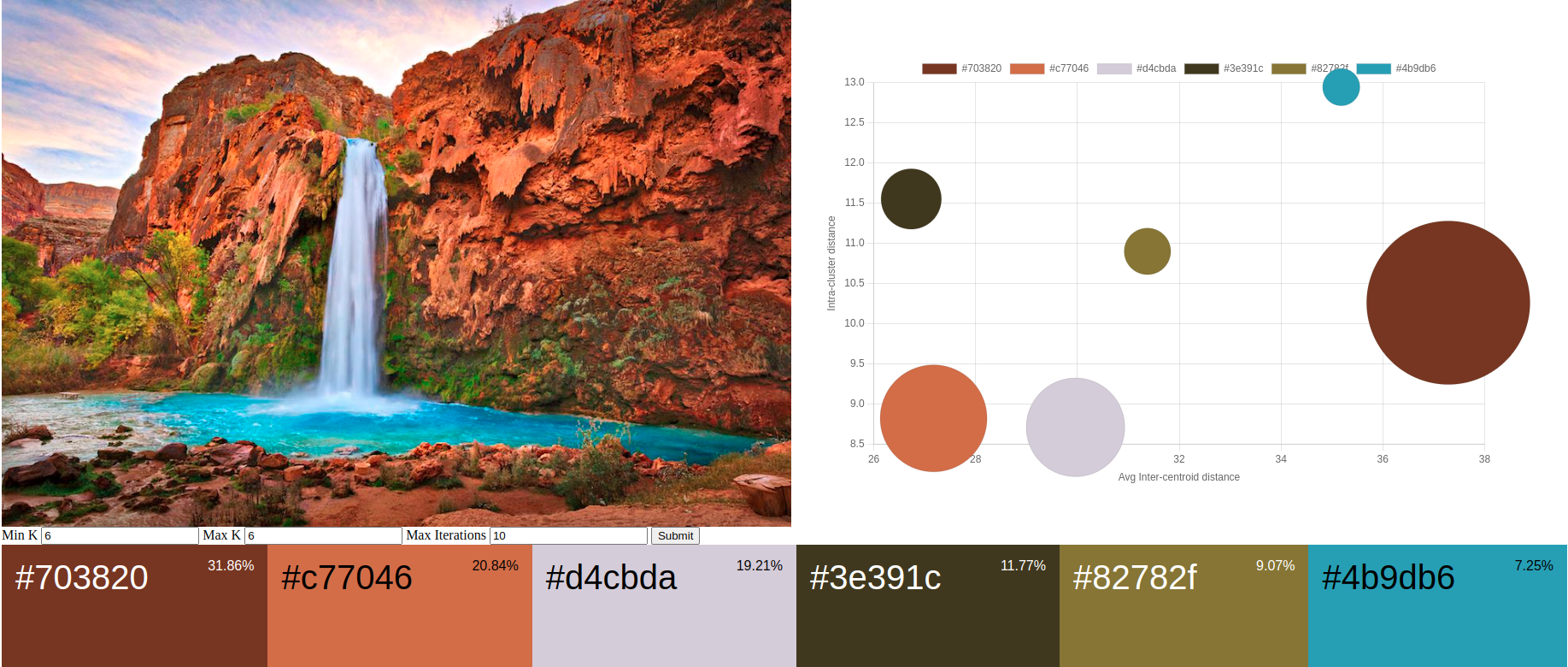
The next step is to present the clusters and evaluation in a meaningful and visually appealing way. One common approach is to create a color palette that showcases the dominant colors alongside the original image.

To create a color palette, you can display the extracted dominant colors as individual color swatches or rectangles, arranged in a grid or a horizontal/vertical layout. Each color swatch should be labeled with its corresponding CIELAB or RGB color values, allowing for precise color identification and reproduction. By presenting the extracted dominant colors in a well-organized color palette, viewers can easily understand and appreciate the key colors that contribute to the overall visual composition of the image.

In addition to the color swatches, it’s helpful to include the percentage or proportion of each dominant color in the image. This information provides insights into the relative prominence of each color and can be displayed as a percentage value or a visual representation, such as a pie chart or bar graph. Bubble graphs can be very effective for visualizing the inter-centroid distance and intra-cluster distance along with the proportion of each dominant color.

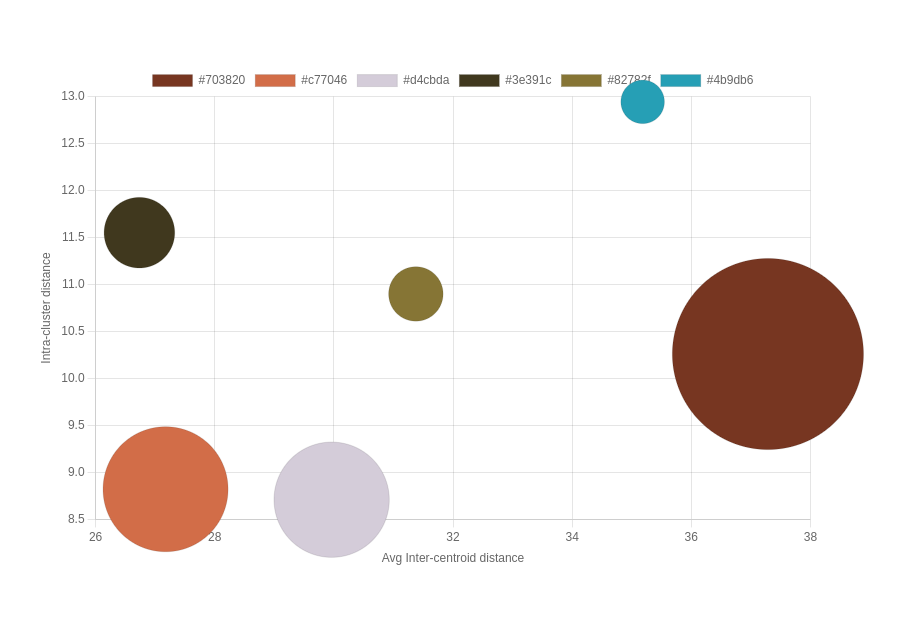
The distances between the bubbles represent the average inter-centroid distances between clusters, with larger distances indicating well-separated and distinct clusters in the perceptual color space, while smaller distances suggest closer proximity and potential overlap or similarity between clusters. The size of each bubble represents the number of data points within each cluster, with smaller bubbles indicating fewer data points and larger bubbles indicating more data points. The average distance to the centroid within each cluster, represented by labels or annotations, provides information about the compactness of each cluster, with smaller distances suggesting tightly grouped and homogeneous data points, and larger distances indicating more spread out and variable data within the cluster.

A dashboard to display the generated color palette with a bubble chart showing the cluster/centroid relationships provide users with a comprehensive overview of the clustering results. Users can quickly grasp the overall color scheme and appreciate the aesthetic qualities of each palette. Alongside the color palette, a bubble chart offers a powerful tool for evaluating the clustering structure and characteristics. Each bubble represents a color cluster, with its size indicating the number of pixels within the cluster and its position reflecting the cluster’s centroid in the perceptual color space. The distances between the bubbles represent the average inter-centroid distances, allowing users to assess the separation and distinctiveness of the color clusters. Additionally, the average distances to the centroids within each cluster are displayed, providing insights into the compactness and homogeneity of the colors within each cluster. By interacting with the bubble chart, users can explore the relationships between color clusters, identify potential outliers or anomalies, and make informed decisions about the quality and suitability of the generated color palette. A simple dashboard’s intuitive and visually engaging presentation of color palettes and clustering evaluation empowers users to analyze, compare, and tune the parameters to the XMeans clustering algorithm.

Applications and Use Cases🔗

• Color palette extraction: By applying X-means clustering with the deltaE2000 metric to an image, you can effectively extract a representative color palette. This is useful for graphic designers, artists, or anyone working with color schemes, as it helps identify the dominant colors in an image while considering human color perception.
• Image compression: Clustering pixels using X-means with deltaE2000 can be used for image compression. By reducing the number of colors in an image to a smaller set of representative colors, you can decrease the image file size while maintaining perceptual quality. This is particularly useful for web graphics or applications where bandwidth is limited.
• Color-based image retrieval: X-means clustering with deltaE2000 can be used to build a color-based image retrieval system. By clustering images based on their dominant colors, you can quickly search and retrieve visually similar images from a large database. This is useful for applications like visual search engines, image recommendation systems, or content-based image retrieval.
• Color harmony analysis: By applying X-means clustering with deltaE2000 to a collection of appeal images, you can analyze color harmony patterns and discover common color combinations that are visually appealing. This information can be valuable for designers, marketers, or researchers studying color psychology and aesthetics.
• Color-based anomaly detection: In industrial or scientific applications, X-means clustering with deltaE2000 can be used to detect color-based anomalies or defects in images. By comparing the color distribution of a test image to a reference image or a cluster model, you can identify regions or pixels that deviate significantly from the expected color range, indicating potential defects or abnormalities.
• Theme-based user interfaces: : Use X-means clustering with deltaE2000 to dynamically theme user interfaces that adapt to the color scheme of user-provided images. By extracting dominant colors from an image and applying them to UI elements, you can create personalized interfaces that match the user’s aesthetic preferences or the content they are interacting with.

Conclusion🔗

The benefits of using X-Means clustering with CIE2000 are clear. This technique not only automatically determines the optimal number of color clusters but also ensures that the resulting color palettes are perceptually meaningful and closely aligned with human color perception. The ability to extract dominant colors accurately opens up a wide range of possibilities in various domains, from data-driven design and image compression to object recognition and data visualization.

To encourage further exploration and experimentation, I’ve provided code implementations for each key component of the dominant color extraction process. These implementations serve as a starting point for readers to dive deeper into the world of color clustering and image processing. We invite you to adapt, modify, and enhance these code snippets to suit your specific needs and explore the limitless potential of this technique.

The significance of perceptually accurate color clustering becomes evident that this approach is not merely an academic exercise but a powerful tool with real-world implications. In a world increasingly driven by visual data, the ability to extract meaningful color information from images is crucial. By embracing techniques like X-Means clustering and CIE2000 color distance, we can create visually stunning designs based on human perception.

References and Further Reading🔗

• X-means extending K-means with Efficient Estimation of the Number of Clusters
• The CIEDE2000 Color-Difference Formula: Implementation Notes, Supplementary Test Data, and Mathematical Observations
• CIE
• Color difference
• The development of the CIE 2000 colour‐difference formula: CIEDE2000