Data Forecasting Math Running

Hierarchical Machine Learning Classification Tasks

May 12th, 2020

Machine learning models have varying levels of accuracy which needs to be accounted for in production environments. By using a threshold-constrained hierarchy, we can make predictions based on membership probability to subsets of classes.

Home Projects

Overview🔗

Trained machine learning models are rarely 100% accurate when making predictions in any real-world task. This post describes the steps/tradeoffs that I took to minimize the number of mistakes that are made by a machine learning classifier and to maximize the utility of the classifier. This method can be used when stakeholders have a low-tolerance for errors in the domain of the machine learning classification. This method involves creating a class taxonomy, and creating thresholds at which a classification can be assigned or acted upon. The taxonomy, in combination with action thresholds, allows the developer to optimize the balance the risk tolerance of the stakeholders with efficiency of the process. By setting a higher confidence threshold for acting on a classification, fewer actions are taken but the actions that are taken should tend to be accurate. If the the threshold for action is lower, more actions will be taken, but the classifications may not be accurate.

Taxonomy🔗

The simplest machine learning classification tasks involve directly classifying samples into classes. This approach to classification relies exclusively on the ability of the model to identify the class of the sample. Many situations can involve classifying samples into one of hundreds or thousands of classes which can be difficult for these flat machine learning models to accurately predict. But making actionable predictions does not always require being able to classify samples into a specific class, but instead being able to determine if the samples are a member of any of a subset of classes that are similar. If a subset of those classes are similar in ways that can be acted on, they can be thought of as the same class. That subset of classes are said to form a higher level class. Higher level classes can be merged into even higher level classes, creating multiple layers of classes. In the context of hierarchical classification, these layers of classes are called a taxonomy of classes. Those classes from which all higher level classes are derived from are called leaf classes, in that they are the lowest and most specific classes in the taxonomy.

The taxonomy of classes allows action to be taken on these higher level classifications, even in the absence of good leaf classifications. For example, if we were trying to classify images of animals, the model may not accurately differentiate between a mountain lion and a house cat. However, depending on what our model is being used for, being able to identify the animal as a feline or as a mammal may be all that is needed to act on the data. If a flat approach were used, the model may end up providing falsely identifying the house cat as a mountain lion, resulting in only inaccurate information. But if a hierarchical classification approach were used, the model could still accurately label the animal as a mammal and a feline, even if the species is still wrong.

Taxonomies are often structured as trees, where lower-level classes are in a direct subset of one higher level class, but they can also be structured as Directed Acyclic Graphs (DAGs), where they are in the direct subset of multiple higher-level graphs. DAGs offer more flexibility and options for structuring higher-level classes, but makes making predictions much more difficult. I would recommend sticking to trees when first starting to work with hierarchical classification.

In a situation with low margin for error, a neural network was being applied using a flat classification classification where it was yielding low accuracy. By refactoring the prediction process into a hierarchical classification approach using the global classifier, actionable predictions increases by 35% by creating a taxonomy of classes which could be used to route information throughout the departments. The taxonomy used was structured similarly to the taxonomy below:

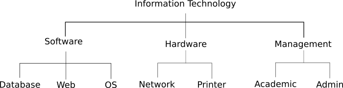
Below is the full Python code for loading, saving, constructing, and traversing our classification taxonomy:

from collections import defaultdict
 
 
class Taxonomy:
    """
    A rooted tree of class labels, e.g.:
 
        Information Technology
        ├── Hardware
        │   ├── Network
        │   └── Printer
        ├── Software
        │   ├── Database
        │   ├── OS
        │   └── Web
        └── Management
            ├── Academic
            └── Admin
 
    Build it with edges:
 
        taxonomy = Taxonomy(root="Information Technology")
        taxonomy.add_edge("Information Technology", "Hardware")
        taxonomy.add_edge("Hardware", "Network")
        ...
    """
 
    def __init__(self, root):
        self.root = root
        self._children = defaultdict(list)   # node -> [children]
        self._parent = {root: None}           # node -> parent (None for root)
 
    def add_edge(self, parent, child):
        if parent not in self._parent:
            raise ValueError(f"{parent!r} has not been added to the taxonomy yet")
        if child in self._parent:
            raise ValueError(f"{child!r} already has a parent ({self._parent[child]!r})")
        self._children[parent].append(child)
        self._parent[child] = parent
 
    def children(self, node):
        return self._children[node]
 
    def is_leaf(self, node):
        return not self._children[node]
 
    def leaves(self):
        return [node for node in self._parent if self.is_leaf(node)]
 
    def parent(self, node):
        return self._parent[node]
 
    def ancestors(self, node):
        """Root-first list of ancestors, not including `node` itself."""
        path = []
        current = self._parent[node]
        while current is not None:
            path.append(current)
            current = self._parent[current]
        return list(reversed(path))
 
    def path_to_root(self, node):
        """Root-first list of nodes from the root down to and including `node`."""
        return self.ancestors(node) + [node]
 
    def depth(self, node):
        """Depth of `node`, where the root is depth 0."""
        return len(self.ancestors(node))
 
    @classmethod
    def from_dict(cls, root, edges):
        """
        Build a Taxonomy from {parent: [children, ...]}.
 
            Taxonomy.from_dict("Information Technology", {
                "Information Technology": ["Hardware", "Management", "Software"],
                "Hardware": ["Network", "Printer"],
                "Management": ["Academic", "Admin"],
                "Software": ["Database", "OS", "Web"],
            })
        """
        taxonomy = cls(root)
        # add parents before their children, in breadth-first order,
        # so add_edge never sees a child before its parent exists
        queue = [root]
        while queue:
            parent = queue.pop(0)
            for child in edges.get(parent, []):
                taxonomy.add_edge(parent, child)
                queue.append(child)
        return taxonomy

But after creating our hierarchy, our process was still assigning inaccurate leaf classes in addition to our accurate higher-level classes. I decided to move away from this mandatory lead-node prediction (MLNP) and move towards non-mandatory leaf-node prediction (NMLNP), where the hierarchical classifier is not required to return a leaf node as the prediction. To systematically limit assigning inaccurate classes, I added thresholds for node prediction assignments, by classifying samples to the lowest ancestor in the taxonomy which exceeds the threshold. By creating this taxonomy of classifications relating to our machine learning model, action can still be taken on samples that the model could not verify with a high degree of certainty.

Putting it all Together🔗

We compute the probabilities of these parent classifications by summing the probabilities of the immediate children of a parent classification. If this computed probability is greater than the threshold, we classify the sample to that parent classification, as it is the lowest classification in the taxonomy that exceeds our threshold. If not, we look at the parent of that classification, and perform the same calculations and comparison to the threshold. If we continue this process until we get to the root classification without exceeding a threshold we do not classify the sample at all.

In the below example, the machine learning classifier did not produce predictions that exceeded any of the classifications (.0.70), so we sum the probabilities for the child classifications of each parent, and assign that value as the probability for that parent. We then compare the parent probabilities to the threshold, and find that the sample can be assigned to “Hardware”, which exceed the threshold. If no parent probability exceeded the threshold, we would not take any action, as the parent of the Software, Hardware, and Management classifications is the root of the taxonomy.

Let’s examine the code that will handle these threshold comparisons, and traversal of our hierarchy.

import logging

logger = logging.getLogger(__name__)


class HierarchicalClassifier:
    """
    Converts leaf-class probabilities into a single prediction by climbing
    the taxonomy: a node's probability is the sum of its leaf descendants'
    probabilities. Starting at the root, keep descending into the child with
    the highest probability as long as that probability clears the
    threshold; stop and return the current node as soon as it doesn't.
 
    args:
        taxonomy (Taxonomy): the class hierarchy to classify into
        threshold (float): minimum probability required to descend into a
            child node. Defaults to 0.0, which always descends to a leaf.
    """
 
    def __init__(self, taxonomy, threshold=0.0):
        self.taxonomy = taxonomy
        self.default_threshold = threshold
 
    def _node_probabilities(self, leaf_probabilities):
        """
        Roll leaf probabilities up the tree: every node's probability is the
        sum of the probabilities of the leaves beneath it.
        """
        node_probabilities = defaultdict(float)
        for leaf, probability in leaf_probabilities.items():
            for node in self.taxonomy.path_to_root(leaf):
                node_probabilities[node] += probability
        return node_probabilities
 
    def predict(self, leaf_probabilities, threshold=None, return_path=False):
        """
        args:
            leaf_probabilities (dict): {leaf_class_name: probability}, one
                entry per leaf class in the taxonomy
            threshold (float or dict): minimum probability required to
                descend into a child node. Either:
                  - a single float applied to every node, or
                  - a dict of {node_name: threshold} for nodes that need
                    their own bar, with a "default" entry for everything
                    else, e.g. {"Database": 0.85, "default": 0.6} if a
                    wrong "Database" ticket is costlier than a wrong
                    "Printer" ticket.
                Defaults to the threshold set when this classifier was
                constructed, but can be overridden per call.
            return_path (bool): if True, return the full list of nodes from
                the root down to the prediction instead of just the
                prediction itself
 
        returns:
            str, or list[str] if return_path=True
        """
        if threshold is None:
            threshold = self.default_threshold
        node_probabilities = self._node_probabilities(leaf_probabilities)
 
        path = [self.taxonomy.root]
        current = self.taxonomy.root
        while not self.taxonomy.is_leaf(current):
            children = self.taxonomy.children(current)
            best_child = max(children, key=lambda child: node_probabilities[child])
            required = self._threshold_for(best_child, threshold)
            if node_probabilities[best_child] < required:
                logger.debug(
                    "stopping at %r: best child %r has probability %.4f, "
                    "below required %.4f",
                    current, best_child, node_probabilities[best_child], required,
                )
                break
            logger.debug(
                "descending %r -> %r (probability %.4f >= required %.4f)",
                current, best_child, node_probabilities[best_child], required,
            )
            current = best_child
            path.append(current)
 
        logger.debug("prediction: %r (depth %d)", current, len(path) - 1)
        return path if return_path else current
 
    @staticmethod
    def _threshold_for(node, threshold):
        """Resolves a float-or-dict threshold down to the value for `node`."""
        if isinstance(threshold, dict):
            if node not in threshold and "default" not in threshold:
                logger.warning(
                    "no threshold entry or 'default' for node %r; "
                    "falling back to 0.0, which always allows descent into it",
                    node,
                )
            return threshold.get(node, threshold.get("default", 0.0))
        return threshold
 
    def predict_batch(self, samples, threshold=None, return_path=False):
        """Apply predict() to a list of {leaf_class: probability} dicts."""
        effective_threshold = self.default_threshold if threshold is None else threshold
        logger.info(
            "predicting batch of %d samples (threshold=%r)",
            len(samples), effective_threshold,
        )
        predictions = [self.predict(sample, threshold=threshold, return_path=return_path) for sample in samples]
        logger.info("finished batch of %d samples", len(samples))
        return predictions
 
    def evaluate(self, y_true, y_pred):
        """
        Scores predictions in a way that fits non-mandatory leaf-node
        prediction: the classifier is allowed to stop early, so "Hardware"
        when the true label is "Network" isn't wrong, it's just less
        specific. Plain exact-match accuracy would punish that correct but
        conservative call the same as a genuine mistake, and it would also
        reward always predicting the root with 100% accuracy. This report
        separates the two questions instead:
 
          correctness: is the prediction on the path from the root down to
              the true leaf (an ancestor of it, or the leaf itself)?
          specificity: given a correct prediction, how far down the
              taxonomy did it get, as a fraction of the true leaf's depth?
              1.0 means it reached the leaf; 0.0 means it stopped at the
              root.
 
        args:
            y_true (list[str]): the true leaf class for each sample
            y_pred (list[str]): the predicted node for each sample, as
                returned by predict() (may or may not be a leaf)
 
        returns:
            dict with:
                accuracy (float): fraction of predictions on the true path
                mean_specificity (float): average depth reached, as a
                    fraction of true depth, among correct predictions
                leaf_rate (float): fraction of predictions that reached a
                    leaf at all (correct or not)
                by_predicted_depth (dict): {depth: {count, accuracy}} -
                    how many predictions stopped at each depth of the
                    taxonomy, and how often those were correct. Useful for
                    seeing which levels the threshold is actually settling
                    predictions at.
        """
        total = len(y_true)
        correct = 0
        specificities = []
        leaf_count = 0
        by_depth = defaultdict(lambda: {"count": 0, "correct": 0})
 
        for true_leaf, prediction in zip(y_true, y_pred):
            true_path = set(self.taxonomy.path_to_root(true_leaf))
            is_correct = prediction in true_path
            predicted_depth = self.taxonomy.depth(prediction)
            true_depth = self.taxonomy.depth(true_leaf)
 
            by_depth[predicted_depth]["count"] += 1
            if is_correct:
                correct += 1
                by_depth[predicted_depth]["correct"] += 1
                specificities.append(predicted_depth / true_depth if true_depth else 1.0)
            if self.taxonomy.is_leaf(prediction):
                leaf_count += 1
 
        report = {
            "accuracy": correct / total,
            "mean_specificity": (sum(specificities) / len(specificities)) if specificities else 0.0,
            "leaf_rate": leaf_count / total,
            "by_predicted_depth": {
                depth: {"count": info["count"], "accuracy": info["correct"] / info["count"]}
                for depth, info in sorted(by_depth.items())
            },
        }
        logger.info(
            "evaluated %d samples: accuracy=%.3f mean_specificity=%.3f leaf_rate=%.3f",
            total, report["accuracy"], report["mean_specificity"], report["leaf_rate"],
        )
        return report
 
 
def threshold_curve(taxonomy, samples, y_true, thresholds):
    """
    Evaluates a HierarchicalClassifier at each threshold in `thresholds`,
    so you can see the accuracy/specificity tradeoff directly instead of
    guessing at a single threshold. This is the risk-tolerance-vs-efficiency
    curve: low thresholds push predictions toward leaves (more specific,
    more likely wrong); high thresholds push predictions toward the root
    (less specific, more likely right).
 
    args:
        taxonomy (Taxonomy): the class hierarchy to classify into
        samples (list[dict]): leaf-class probabilities for each sample
        y_true (list[str]): the true leaf class for each sample
        thresholds (list[float]): thresholds to evaluate
 
    returns:
        list[dict]: one evaluate() report per threshold, each with a
            "threshold" key added
    """
    classifier = HierarchicalClassifier(taxonomy)
    rows = []
    for threshold in thresholds:
        y_pred = classifier.predict_batch(samples, threshold=threshold)
        report = classifier.evaluate(y_true, y_pred)
        rows.append({"threshold": threshold, **report})
    return rows

def hierarchical_prf(taxonomy, y_true, y_pred):
    """
    Scores predictions using the hierarchical precision/recall/F-measure of
    Kiritchenko et al. (2006): the standard, literature-comparable metric for
    hierarchical classification. Each prediction and true leaf is expanded
    into the full set of its ancestors (excluding the root, which every
    sample shares), and precision/recall are computed over the overlap of
    those sets across the whole dataset, rather than per-sample.

    This gives credit for partial correctness in a way plain accuracy can't:
    predicting "Hardware" when the true leaf is "Network" contributes partial
    overlap rather than being scored as flatly wrong. Unlike evaluate(),
    though, it collapses correctness and specificity into a single set of
    numbers; it can't tell you whether wrong predictions landed on the right
    branch at all, or which depth the threshold is actually settling
    predictions at. Use this alongside evaluate() rather than in place of it:
    this is the metric to report for comparison with published results,
    evaluate() is the diagnostic for tuning your own threshold.

    args:
        taxonomy (Taxonomy): the class hierarchy to classify into
        y_true (list[str]): the true leaf class for each sample
        y_pred (list[str]): the predicted node for each sample, as
            returned by predict() (may or may not be a leaf)

    returns:
        dict with:
            hP (float): hierarchical precision - fraction of predicted
                ancestors (across all samples) that were also true ancestors
            hR (float): hierarchical recall - fraction of true ancestors
                (across all samples) that were also predicted
            hF (float): harmonic mean of hP and hR
    """
    intersection = predicted_total = true_total = 0
    for true_leaf, prediction in zip(y_true, y_pred):
        predicted_set = set(taxonomy.path_to_root(prediction)[1:])  # drop root
        true_set = set(taxonomy.path_to_root(true_leaf)[1:])
        intersection += len(predicted_set & true_set)
        predicted_total += len(predicted_set)
        true_total += len(true_set)
    hP = intersection / predicted_total if predicted_total else 0.0
    hR = intersection / true_total if true_total else 0.0
    hF = (2 * hP * hR / (hP + hR)) if (hP + hR) else 0.0
    return {"hP": hP, "hR": hR, "hF": hF}

Let’s show an example of how you might use this HierarchicalClassifierin a real-world scenario:

taxonomy = Taxonomy.from_dict("Information Technology", {
    "Information Technology": ["Hardware", "Management", "Software"],
    "Hardware": ["Network", "Printer"],
    "Management": ["Academic", "Admin"],
    "Software": ["Database", "OS", "Web"],
})
 
classifier = HierarchicalClassifier(taxonomy, threshold=0.60)
 
samples = [
    {"Database": 0.0752, "OS": 0.08, "Web": 0.22, "Network": 0.45,
        "Printer": 0.18, "Academic": 0.0045, "Admin": 0.003},
    {"Database": 0.01, "OS": 0.3, "Web": 0.0, "Network": 0.091,
        "Printer": 0.05, "Academic": 0.0, "Admin": 0.0},
    {"Database": 0.15, "OS": 0.15, "Web": 0.15, "Network": 0.15,
        "Printer": 0.15, "Academic": 0.15, "Admin": 0.10},
]
 
for sample in samples:
    print(classifier.predict(sample))
# Hardware  (Network 0.45 alone misses 0.60, but Hardware = 0.45+0.18 = 0.63)
# Information Technology  (nothing clears 0.60 even at the top level)
# Information Technology  (probabilities are too spread out)
 
# the true leaf class for each sample above
y_true = ["Network", "OS", "Database"]
y_pred = classifier.predict_batch(samples)
print(classifier.evaluate(y_true, y_pred))  # {'accuracy': 1.0, 'mean_specificity': 0.16666666666666666, 'leaf_rate': 0.0, 'by_predicted_depth': {0: {'count': 2, 'accuracy': 1.0}, 1: {'count': 1, 'accuracy': 1.0}}}
 
print()
for row in threshold_curve(taxonomy, samples, y_true, thresholds=[0.0, 0.3, 0.5, 0.6, 0.7, 0.9]):
    print(f"threshold={row['threshold']:.1f}  "
            f"accuracy={row['accuracy']:.2f}  "
            f"specificity={row['mean_specificity']:.2f}  "
            f"leaf_rate={row['leaf_rate']:.2f}")
 
# A sample where Database alone clears the default 0.60 threshold, so the
# per-node override actually has something to bite on
database_leaning_sample = {"Database": 0.65, "OS": 0.05, "Web": 0.05, "Network": 0.10,
    "Printer": 0.05, "Academic": 0.05, "Admin": 0.05}
override_samples = samples + [database_leaning_sample]
 
# Database tickets need higher confidence than everything else before
# they're assigned directly; everything else uses the default 0.60
strict_database_threshold = {"Database": 0.85, "default": 0.60}
 
print()
print("default threshold (0.60 everywhere):     ", classifier.predict_batch(override_samples))
print("strict Database threshold (0.85 for it): ", classifier.predict_batch(override_samples, threshold=strict_database_threshold))
# default threshold (0.60 everywhere):      ['Hardware', 'Information Technology', 'Information Technology', 'Database']
# strict Database threshold (0.85 for it):  ['Hardware', 'Information Technology', 'Information Technology', 'Software']

Benefits and Limitations🔗

Benefits🔗

The HierarchicalClassifier approach has a few benefits:

• Reusability: the HierarchicalClassifierdoes not interact directly with the model, only the output probabilities. It can be used with any machine learning framework, any neural network architecture, or any set of labeled probabilities.
• Taxonomy agnostic: The implementation will work with any taxonomy containing the classes predicted by the classifier, so the number of layers in the taxonomy will not make a difference when making classifications. This also means that the same classifier can be used in multiple hierarchies, allowing developers to swap hierarchies in/out of the implementation at runtime.
• Dynamic: This implementation allows hierarchies to built and altered at runtime, so the developer can use other techniques to dynamically build the optimal taxonomy from a database, or restructure the taxonomy to meet the needs of their situation. It also allows for developers to build interfaces for non-technical stakeholders to build/modify the taxonomy and thresholds without developers.

Limitations🔗

• Error propagation: predict() is greedy. At each level it descends into whichever single child scored highest, and never reconsiders that choice once made. If “Software” narrowly out-scores “Hardware” at the top level even though the true leaf is “Network,” the classifier commits to “Software” and can never reach “Network,” no matter how strong the evidence for it was further down the tree. Tuning the threshold doesn’t fix this: the threshold only controls how far an already-chosen branch is followed, not whether the right branch was chosen in the first place. This is commonly called error propagation in the hierarchical classification literature. A mistake made high in the tree can’t be undone by information available deeper in it. Methods that jointly optimize the full path through the tree, rather than committing one level at a time, avoid this at the cost of considerably more complexity.
• Calibration and mutual exclusivity: _node_probabilities() computes a parent’s probability by summing the probabilities of its leaf descendants. That sum only means something if the underlying leaf probabilities are mutually exclusive and sum to (approximately) 1 across the whole leaf set (the output of a softmax, for instance). If the leaf probabilities instead come from independent per-class scores, as is common with multi-label or sigmoid-based models, the sums this classifier relies on won’t correspond to any real “probability of being in this subtree,” and the threshold comparisons will silently produce meaningless results. So Before plugging a new model’s output into this classifier, check that its leaf probabilities are calibrated and sum to 1.

UPDATE: After implementing this code (and this post) I discovered that there was already a whole field of study dedicated to this problem. I went ahead and updated this post to reflect the language used in that research. If you are interested in diving deeper into methods of hierarchical classification, I would recommend A survey of hierarchical classification across different application domains to get a high level overview of hierarchical classification techniques and advantages/disadvantages to each.

Further Reading🔗

This post covers one specific technique: threshold-based climbing on top of an already-trained flat classifier. This is especially useful in scenarios where you can’t train your own models, or can’t dedicate more resources to training. But it’s a small corner of a much larger body of work, Here are some further resources if you want to pursue hierarchical classification further:

• A survey of hierarchical classification across different application domains (Silla & Freitas, 2011): The paper referenced throughout this post. It’s the best starting point for understanding the field as a whole: it defines what counts as hierarchical classification, and proposes the framework this post borrows terminology from for categorizing approaches (flat vs. local classifier vs. global classifier).
• Learning and Evaluation in the Presence of Class Hierarchies: Application to Text Categorization (Kiritchenko, Matwin, Nock & Famili, 2006): Introduces hierarchical precision, recall, and F-measure: an extension of ordinary precision/recall that credits partially-correct predictions based on shared ancestors, rather than scoring only exact leaf matches. Complements (rather than replaces) the accuracy/specificity/leaf_rate metrics used in this post’s evaluate() — the former is the standard, literature-comparable score; the latter is a better diagnostic for tuning your threshold.
• Evaluation measures for hierarchical classification: a unified view and novel approaches (Kosmopoulos, Partalas, Gaussier, Paliouras & Androutsopoulos, 2014): Later survey specifically of hierarchical evaluation measures, useful if you want a broader comparison of metric families beyond Kiritchenko et al.
• Making Better Mistakes: Leveraging Class Hierarchies with Deep Networks (Bertinetto, Mueller, Tertikas, Samangooei & Lord, 2020): Proposes modifications to the cross-entropy loss so that a model is penalized more for mistakes that are further away in the class hierarchy (confusing a house cat for a mountain lion) than for mistakes that are nearby (confusing a house cat for a raccoon). It changes what the model learns, rather than reasoning over the output of a model that was trained flat. Worth reading if the flat classifier feeding into HierarchicalClassifier is itself something you are able to control and can retrain.