Graph-theory Math Python

Network Science - Node Strength, Centrality and Communicability

An introduction to Hirsch index-based metrics for measuring node importance in weighted graphs based on degrees and node strengths, and a centrality for measuring communication ability of a node in a network.

Home Blog

Overview🔗

H-degrees are a fast, edge-based distribution measure in weighted networks that capture more of it’s structural properties than node degree or edge weights, and can make distinctions that node degrees and edge weights individually cannot. H-degrees have applications in any discipline and can be applied to any weighted network. H-degree is also used to create the communication centrality, which, unlike many other network centralities, can be applied to networks that do not have geodesic flows.

This post will also cover methods based on the H-degree that can be used to measure and compare networks by their distribution of edges and edge weights.

In this post I will cover the following measures:

• Lobby Index
  • w-Lobby Index
  • Lobby Gain
  • l-core
• G-index
• H-degree
  • In-H-degree
  • Out-H-degree
  • H-degree centrality
  • H-centralization
  • H-ratio index
• Communication Centrality
  • \(C_c\) -centrality
  • c-core nodes
  • c-centralization

Lobby Index🔗

The first measure of node strength was the Hirsch Index for measuring the output of an academic scholar in terms of publications and citations. This metric inspires all of the metrics that are in this post and their calculations are based on those of the Hirsch Index.

A scientist has index \( h \) if \( h \) of his or her \( N \) papers have at least \( h \) citations each and the other \( N - h \) papers have \( h \) or fewer citations each

The following _h_index_helper function is a function that computes the h-index on a given iterable of values, and will be used throughout this post to significantly shorten implementations of h-index-like metrics.

def _h_index_helper(iterable, sorted=False):
    if not isinstance(iterable, list):
        iterable = list(iterable)
    if not sorted:
        iterable.sort()

    value_count = len(iterable)
    for index, value in enumerate(iterable):
        result = value_count - index
        if result <= value:
            return result

    return 0

Here is an implementation of the H-index:

def h_index(G, node):
    """
    The Hirsch Index
    Parameters
    ----------
    G: graph
        A networkx Graph
    node: object
        A node in the networkx graph

    Returns
    -------
    int:  the H-index of the given node
    """
    neighbors = list(G.neighbors(node))
    degrees = list(degree for n, degree in G.degree(neighbors))
    return _h_index_helper(degrees)

This measure was later the inspiration for the lobby index, which is a generalization of the Hirsch index to be applied to any weighted or unweighted network. Formally, the lobby index is defined as

The l-index or **lobby index** of a node \( n \) is the largest integer \( k \) such that \( n \) has at least \( k \) neighbors with a degree of at least \( k \)... $$ l(n) = \max{\{ k: deg(y_k) \geq k \}} $$ such that all \( y_k \) are neighbors of node \( n \)

The lobby index is called a lobby index because it is a quantified indicator for how strong a node’s lobbying/influence is in a network both in terms of number of neighbors a node has and how highly connected their neighbors are. So, to put it simply, the lobby index is based on the degree distribution of a node’s direct neighbors. This makes the lobby index useful for identifying strong/weak nodes based on the degree distribution of it’s neighbors, such as in communication networks and social networks, or political influence networks.

It is clear that a person has strong lobby power, the ability to influence people’s opinions, if he or she has many highly connected neighbors. This is exactly the aim of a lobbyist or a diplomat. The diplomat’s goal is to have strong influence on the community while keeping the number of his connections (which have a cost) low. If \( x \) has a high lobby index, then the l-core \( L(x) \) (those neighbors which provide the index) has high connectivity.

l-core nodes are the neighbor nodes that contribute to the lobby index of a node. The author also provides a metric called lobby gain which shows how the access to the network is multiplied using a link to the l-core nodes. The lobby gain can be determined using the following equation:

\[\Gamma_l(x) = \Large{deg_2^L(x) \over l(x) }\]

where ( deg_2^L(x) ) is the number of second neighbors reachable via the l-core nodes of ( x ). These formulas quantify the effects of a neighborhood’s degree distribution on a node’s ability to access the rest of the network. The lobby gain quantifies a node’s accessibility to the network through it’s most important connections and makes the connections of different nodes comparable in terms of connectivity. Between the lobby index and the lobby gain, developers can identify the high-degree neighbors of a node and quantify the access that they provide to the network.

The lobby-index has a moderate correlation with closeness, betweenness and eigenvector centrality. The distribution of the lobby index can be approximated to be the following in a scale-free network:

\[P( l(x) \geq k) \eqsim k^{-\alpha(\alpha + 1)}\]

where ( \alpha ) is the tail exponent of the degree distribution. If a node has many neighbors with high-degree it has a high lobby index. But how so we know if a given lobby-index is good? The author of the original paper gives the reader the following equation to evaluate a lobby index in a scale-free network:

\[l(x) \approx c deg(x)^{1 \over{\alpha + 1}}\]

where ( c ) is a constant.

An alternative to the lobby index in weighted graphs is the weighted lobby index, or w-lobby index. The w-lobby index accounts for the number of connections a node has, and the strength of relationships that those neighbors have via their edge weights. The strength of relationships a node has with it’s neighbors is called it’s node strength. Node strength is the sum of the weights of edges to/from a node.

the w-lobby index (weighted network lobby index) of node \( n \), is defined as the largest integer \( k \) such that node \( n \) has at least \( k \) neighbors with node strength at least \( k \).

I have been able to find remarkably little research on the w-lobby index, so I won’t dedicate anymore time/space to this measure.

The following code implements the node_strength, lobby index, and l-core calculations.

def node_strength(G, node, attribute):
    """
    Node strength is defined as the sum of the strengths (or weights) of all
    of the nodes edges.

    Parameters
    ----------
    G: graph
       A networkx graph
    node: object
       A node in the networkx graph
    attribute: object
       The edge attribute used to quantify node strength

    Returns
    -------
    node strength: (int, float)
    """
    output = 0.0
    for edge in G.edges(node):
        output += G.get_edge_data(*edge)[attribute]
    return output


def l_core(G, node, attribute=None, l_index=None):
    """
    Parameters
    ----------
    G: graph
       A networkx graph
    node: object
        Node to calculate the C-core nodes of
    attribute: object
        The edge attribute used to determine strength of a node
    l_index: int
        The lobby index of the given node

    Returns:
        set: L-core nodes of the given node in the given graph

    References
    ----------
    .. [1]  A. Korn, A. Schubert, A. Telcs, Lobby index in networks,
       Physica A 388 (11) (2009) 2221–2226.
       https://arxiv.org/abs/0809.0514
    """
    if not l_index:
        l_index = lobby_index(G, node, attribute)
    output = set()
    for neighbor in G.neighbors(node):
        if attribute:
            value = node_strength(G, neighbor, attribute)
        else:
            value = G.degree(neighbor)
        if value >= l_index:
            output.add(neighbor)

    return output


def lobby_index(G, node, attribute=None):
    """
    Parameters
    ----------
    G: graph
       A networkx graph
    node: object
       A node in the networkx graph
    attribute: object
       The edge attribute used to determine node strength for a weighted lobby
       index, defaults to None to use node degree to compute the unweighted
       lobby index

    Returns
    -------
    lobby index: int
    """
    if attribute:
        """
        w-lobby index:
        largest integer k such as the node has at least k neighbors with node
        strength at least k
        """
        values = [node_strength(G, n, attribute) for n in G.neighbors(node)]
    else:
        """
        The lobby index of a node in an unweighted graph is defined as the
        largest integer k such that the node has at least k neighbors with a
        degree of at least k
        """
        values = [value for n, value in G.degree(G.neighbors(node))]
    return _h_index_helper(values)

Here is an example of how to use the lobby_index function

 data = (
    ('A', 'B', 3),
    ('A', 'C', 5),
    ('A', 'D', 1),
    ('A', 'E', 3),
    ('B', 'F', 1),
    ('C', 'F', 2),
)
nodes = 'ABCDEF'
G = nx.Graph()
G.add_nodes_from(nodes)
for source, target, weight in data:
    G.add_edge(source, target, weight=weight)
    
for node in nodes:
     l_index = lobby_index(G, node)
     w_lobby_index = lobby_index(G, node, 'weight')
     l_core_val = l_core(G, node)
     print('Node: %r, lobby-index: %r, l-core: %r, W-lobby index: %r' % (node, l_index, l_core_val, w_lobby_index))

Update: C-index and G-index🔗

In 2006, Leo Egghe proposed the G-index as an improvement to the h-index was proposed which makes highly connected neighbors of a node benefit increase the index of the node. This makes it a more fair approach than the h-index. However, the g-index becomes saturated when the average number of edges for all nodes exceeds the total number of nodes, which makes it unsuitable for situations where that can occur.

def cg_index(G, node, attribute):
    """
    A g-index based metric evaluating the importance of a node based on the
    product of the strength of neighbor nodes and the strength of the
    connecting edge.
    Parameters
    ----------
    G: graph
       A networkx graph
    node: object
       A node in the networkx graph
    attribute: object
       The edge attribute used to determine node strength for a weighted lobby
       index, defaults to None to use node degree to compute the unweighted
       lobby index
    Returns
    -------
    cg-index: int
    Notes
    -----
    According to [1]_, the :math:`c_g`-index is sourced from the g-index and is
    defined as:
    :math:`c_g` is the highest rank such that the sum of the products of the
    edge strength of the top :math:`c_g` node and the strength of corresponding
    neighbor node is at least :math:`c_g^2`, noted by :math:`c_g(x)`, namely
    :math:`c_g(x) = c_g`.
    :math:`c_g`-index preferentially stresses the importance of edges with
    high strength and neighbor nodes with high node strength, which is fairer
    for low degree nodes and with larger edge strengths or the neighbor
    nodes with large node strengths.
    References
    ----------
    .. [1]  Yan, Xiangbin, Zhaia, Li, Fan., W., 2013. C-index: a weighted
       network node centrality measure for collaboration competence. J.
       Informetr. 7, 223–239.
       https://www.sciencedirect.com/science/article/abs/pii/S1751157712000946
    """
    weights = []
    for neighbor in G.neighbors(node):
        neighbor_strength = node_strength(G, neighbor, attribute)
        weight = G.get_edge_data(node, neighbor)[attribute]
        value = neighbor_strength * weight
        weights.append(value)
    accumulated_product = sum(weights)

    index = 0
    while index ** 2 < accumulated_product:
        index += 1
    return index - 1


def g_index(G, node, attribute):
    """
    An index for evaluating the importance of a node based on the strength of
    it's neighbor nodes, with no degree-based limit.
    Removes the node degree limit on the index value to more fairly evaluate
    low degree nodes with high edge strength or having important neighbors.
    Parameters
    ----------
    G: graph
       A networkx graph
    node: object
       A node in the networkx graph
    attribute: object
       The edge attribute used to determine node strength for a weighted lobby
       index.
    Returns
    -------
    g-index: int
    Notes
    -----
    According to [1]_, g-index is defined as:
    A set of papers has a g-index :math:`g` if :math:`g` is the highest rank
    such that the top :math:`g` papers have, together, at least :math:`g^2`
    citations. This also means that the top :math:`(g + 1)` papers have less
    than :math:`(g + 1)^2` papers.
    References
    ----------
    .. [1]  Egghe, L. (2006). Theory and practise of the g-index.
       Scientometrics, 69(1), 131-152.
       https://link.springer.com/article/10.1007/s11192-006-0144-7
    """
    weights = []
    for neighbor in G.neighbors(node):
        if G.is_directed():
            value = 0.0
            for edge in G.in_edges(neighbor):
                value += G.get_edge_data(*edge)[attribute]
        else:
            value = node_strength(G, neighbor, attribute)
        weights.append(value)
    accumulated_product = sum(weights)

    index = 0
    while index ** 2 < accumulated_product:
        index += 1
    return index - 1

H-Degree🔗

The H-index and lobby index inspired the creation of the H-degree in 2011, which is based on the relationships of a node with its neighbors rather than on the relationships of the node’s neighbors. The H-degree is a measure based on the distribution of edge weights of a given node with it’s neighbors and can be applied to both undirected and directed graphs. The h-degree of a node increases as the node’s degree increases and as the weights of the node’s edges increase.

The h-degree (\( d_h \)) of node \( n \) in a weighted network is equal to \( d_h(n) \) if \( d_h(n) \) is the largest natural number such that \( n \) has at least \( d_h(n) \) links each with strength at least equal to \( d_h(n) \)

The H-degree is correlated with the node degree, but differs to the role of edge weights in the H-degree. Also pictures are the Lobby Index, and w-Lobby Index, and Communication centrality of each node. This graph originally appeared in h-Degree as a basic measure in weighted networks

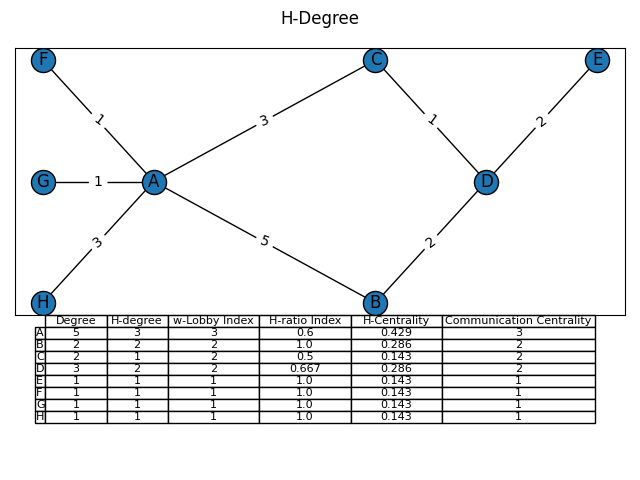
The H-degree can be used in communications network to measure the strength and breadth of a node’s relationships with it’s direct neighbors based purely on the strength of their connecting edges.

Directed H-Degree🔗

In a directed graph, the H-degree can computed for in/out degrees, and is called the In-h-Degree and Out-h-Degree.

**Definition 1**. In a directed weighted network, the In-h-degree (\( h_I \)) of Node \( n \) is equal to \( h_I(n) \) if \( h_I(n) \) is the largest natural number such that \( n \) has at least \( h_I(n) \) In-links each with strength at least equal to \( h_I(n) \). **Definition 2**. In a directed weighted network, the Out-h-degree (\( h_O \)) of Node \( n \) is equal to \( h_O(n) \) if \( h_O(n) \) is the largest natural number such that \( n \) has at least \( h_O(n) \) Out-links each with strength at least equal to \( h_O(n) \).

def hdegree(G, node, attribute, in_edges=False, out_edges=False):
    """
    Parameters
    ----------
    G: graph
       A networkx graph
    node: object
       A node in the networkx graph
    attribute: object
       The edge attribute used to determine strength of a node
    in_edges: boolean
       Indicates if in edges should be considered for a node in a directed
       graph.  If both in_edges and out_edges are the same, both will be
       considered.
    out_edges: boolean
       Indicates if out edges should be considered for a node in a directed
       graph.  If both in_edges and out_edges are the same, both will be
       considered.

    Returns
    -------
    h-degree: int

    References
    ----------
    .. [1]  Zhao, S. X., Rousseau, R., & Ye, F. Y. (2011). H-Degree as a basic
       measure in weighted networks. Journal of Informetrics, 5(4), 668–677.
       https://www.sciencedirect.com/science/article/abs/pii/S1751157711000691

    .. [2]  S.X. Zhao, F.Y. Ye, Exploring the directed h-degree in directed
       weighted networks, Journal of Informetics 6 (2012) 619–630.
       https://www.sciencedirect.com/science/article/pii/S175115771200050
    """
    directed = in_edges ^ out_edges
    if not G.is_directed() and directed:
        raise ValueError("Undirected graphs do not have in/out edges")

    if G.is_directed() and directed:
        if in_edges:
            edge_iterator = G.in_edges(node)
        else:
            edge_iterator = G.out_edges(node)
    else:
        edge_iterator = G.edges(node)

    weights = []
    for edge in edge_iterator:
        weights.append(G.get_edge_data(*edge)[attribute])

    return _h_index_helper(weights)

Here is an example of how to use the hdegree function

data = (
    ('A', 'B', 3),
    ('A', 'C', 5),
    ('A', 'D', 1),
    ('A', 'E', 3),
    ('B', 'F', 1),
    ('C', 'F', 2),
)
nodes = 'ABCDEF'
G = nx.Graph()
G.add_nodes_from(nodes)
for source, target, weight in data:
    G.add_edge(source, target, weight=weight)

for node in nodes:
    hdeg = hdegree(G, node, 'weight')
    print('Node: %r, H-degree: %r' % (node, hdeg))

These directed H-degree measures adds a directional component to the H-degree and opens the door to comparing the in/out H-degree measures using the ( H_{dif} ).

**Definition 5.** In a directed weighted network with \( N \) nodes ( \( N > 1 \) ), the h-difference \( (h_{dif}(n) ) \) of node \( n \) is defined as: $$ h_{dif}(n) = h_I(n) − h_O(n) $$

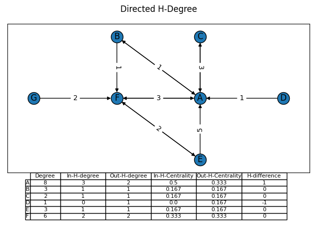
The H-difference can be used to measure the difference between the input to a node, and the output from a node. In a communications network, where nodes represent users and edges represent communications from one user to another, and the edge weight represents the frequency with which they communicate with them. The users who have sent messages to the given user are the input nodes, and the output nodes are those users who the given. If a user has a high in-H-degree and a low out-H-degree, or a negative h-difference, then the user is an information consumer, receiving more communications from more users, and sending fewer emails to fewer users. If a user has a low in-H-degree and a high-H-degree, or a positive h-difference, then they are an information producer, receiving fewer communications from less people, and sending more communications to more users.

H-degree Centrality🔗

H-degree can be used to create a node centrality based on the total number of nodes in the graph:

**Definition 2** In a weighted network with \( N \) nodes, the h-centrality, \( C_h \), of node \( n \) is defined as: $$ C_h(n) = \Large{ d_h(n) \over N − 1} $$ where \( d_h(n) \) is the h-degree of node \( n \). h-Centrality is just a normalized form of the h-degree.

Directed forms of the H-degree centrality are also offered.

**Definition 3** In a directed weighted network with \( N \) nodes ( \( N > 1 \)), the In-h-centrality ( \(C_{hI}(n) \) ) of node \( n \) is defined as: $$ C_{hI}(n) = \Large{ h_I(n) \over N - 1 } $$ **Definition 4** In a directed weighted network with \( N \) nodes ( \( N > 1 \)), the Out-h-centrality ( \(C_{hO}(n) \) ) of node \( n \) is defined as: $$ C_{hO}(n) = \Large{ h_O(n) \over N - 1 } $$

Since both of the directed H-centralities are normalized by the number of nodes in the graph, the In/Out-H centralities of nodes in different graphs, or the same graph over time are comparable. The directed H-degree centralities are subject to the following constraints, which can be used as minimum and maximum values:

**Proposition 1.** In a directed weighted network with \( N \) nodes (\( N > 1 \)), for a non-isolated node \( n \), the following inequalities always hold: $$ 0 \leq C_{hI}(n) \leq \Large{ N_I(n) \over N - 1 } \leq 1 $$ $$ 0 \leq C_{hO}(n) \leq \Large{ N_O(n) \over N - 1 } \le 1 $$

where ( N_I(n) ) denotes the numbers of node ( n )’s neighbor nodes which maintain In-links with node ( n ).

**Proposition 2.** In a directed weighted network with \( N \) nodes (\( N > 1\)), for a non-isolated node \( n \), the following inequalities always hold: $$ C_{hI}(n) \leq \Large{ \sqrt{C_I(n)} \over N - 1 } $$ $$ C_{hO}(n) \leq \Large{ \sqrt{C_O(n)} \over N - 1 } $$ where the \( C_I(n) \) and \( C_O(n) \) denote the in-degree centrality and out-degree centrality, respectively.

def hdegree_centrality(G, attribute, **kwargs):
    """Calculates the hdegree centrality for all nodes in a graph

    Parameters
    ----------
    G: graph
       A networkx graph
    node: object
       A node in the networkx graph
    attribute: object
       The edge attribute used to determine strength of a node

    Keyword Parameters
    ------------------
    in_edges: boolean
       Indicates if in edges should be considered for a node in a directed
       graph.  If both in_edges and out_edges are the same, both will be
       considered.
    out_edges: boolean
       Indicates if out edges should be considered for a node in a directed
       graph.  If both in_edges and out_edges are the same, both will be
       considered.

    Returns
    -------
    dict: H-degree centralities of the nodes in graph G

    References
    ----------
    .. [1]  Zhao, S. X., Rousseau, R., & Ye, F. Y. (2011). H-Degree as a basic
       measure in weighted networks. Journal of Informetrics, 5(4), 668–677.
       https://www.sciencedirect.com/science/article/abs/pii/S1751157711000691

    .. [2]  S.X. Zhao, F.Y. Ye, Exploring the directed h-degree in directed
       weighted networks, Journal of Informetics 6 (2012) 619–630.
       https://www.sciencedirect.com/science/article/pii/S175115771200050
    """
    nodes = G.nodes()
    node_count = len(nodes)
    output = dict()
    denominator = node_count - 1.0
    for node in G.nodes:
        node_hdegree = hdegree(G, node, attribute, **kwargs)
        output[node] = node_hdegree / denominator
    return output

Here is an example of how to use the hdegree_centrality function

data = (
    ('A', 'B', 3),
    ('A', 'C', 5),
    ('A', 'D', 1),
    ('A', 'E', 3),
    ('B', 'F', 1),
    ('C', 'F', 2),
)
nodes = 'ABCDEF'
G = nx.Graph()
G.add_nodes_from(nodes)
for source, target, weight in data:
    G.add_edge(source, target, weight=weight)

hdeg_centrality = hdegree_centrality(G, 'weight')
print(hdeg_centrality)

H-Centralization🔗

The H-degree allows for developers to quantify the edge weight distribution of network in graphs using the H-centralization ( C_h ). If the H-centralization of a network is high, a subset of the nodes in the network have higher degree and higher edge weights than the rest of the network. If the H-centralization is low, then the edges and edge weight are distributed more evenly between all the nodes in the network.

**Definition 3** In a weighted network \( G \) with \( N \) nodes, the h-centralization, $$C_h(G) \) of this network is $$ C_h(G) = \Large{ \sum_{i=1}^N [\text{MAX}(G) - d_h(n_i)] \over (N - 1)(N - 2) } $$ where \( d_h(n) \) is the h-degree of node \( n \). h-Centrality is just a normalized form of the h-degree.

The directed H-centralization measures for directed networks quantify the distribution of In/Out-edges and the edge-weights in In/Out edges. The equations for calculating these measures are very similar to the undirected H-centralization and are quoted from the original paper below:

**Definition 6.** In a directed weighted network with \( N \) nodes (\( N > 1 \)), the In-h-centralization (\( C_{hI}(G) \)) of this network is defined as: $$ C_{hI}(G) = \Large{ \sum_{i=1}^N [\text{MAX}_I(G) - d_{hI}(n_i)] \over (N - 1)^2 } $$ **Definition 7.** In a directed weighted network with \( N \) nodes (\( N > 1 \)), the Out-h-centralization (\( C_{hO}(G) \)) of this network is defined as: $$ C_{hO}(G) = \Large{ \sum_{i=1}^N [\text{MAX}_O(G) - d_{hO}(n_i)] \over (N - 1)^2 } $$ where the \( C_I(n) \) and \( C_O(n) \) denote the in-degree centrality and out-degree centrality, respectively.

These H-centralization measures allow developers to quantify and compare the degree of total centralization, and quantify the in/out centralizations within networks as a method to quantify the differences in distributions of degrees and edge weights between the nodes in networks.

def hdegree_centralization(G, attribute, **kwargs):
    """
    Describes the distribution of edge weights in a network.

    Parameters
    ----------
    G: graph
       A networkx graph
    attribute: object
       The edge attribute used to determine strength of a node

    Keyword Parameters
    ------------------
    in_edges: boolean
       Indicates if in edges should be considered for a node in a directed
       graph.  If both in_edges and out_edges are the same, both will be
       considered.
    out_edges: boolean
       Indicates if out edges should be considered for a node in a directed
       graph.  If both in_edges and out_edges are the same, both will be
       considered.

    Returns
    -------
    float: h-degree centralization of the given graph

    References
    ----------
    .. [1]  Zhao, S. X., Rousseau, R., & Ye, F. Y. (2011). H-Degree as a basic
       measure in weighted networks. Journal of Informetrics, 5(4), 668–677.
       https://www.sciencedirect.com/science/article/abs/pii/S1751157711000691

    .. [2]  S.X. Zhao, F.Y. Ye, Exploring the directed h-degree in directed
       weighted networks, Journal of Informetics 6 (2012) 619–630.
       https://www.sciencedirect.com/science/article/pii/S175115771200050
    """
    directed = kwargs.get("in_edges", False) ^ kwargs.get("out_edges", False)

    if not G.is_directed() and directed:
        raise ValueError(
            "Cannot determine directed h-centralization on a undirected graph"
        )
    hdegrees = [hdegree(G, node, attribute, **kwargs) for node in G.nodes()]
    node_count = G.number_of_nodes()
    n1 = node_count - 1
    if G.is_directed() and directed:
        max_value = max(hdegrees)
        denominator = n1 ** 2
    else:
        max_value = G.number_of_nodes() - 1
        n2 = node_count - 2
        denominator = float(n1 * n2)

    numerator = sum(max_value - value for value in hdegrees)
    return numerator / denominator

The hdegree_centralization function can be used as follows:

data = (
    ('A', 'B', 5),
    ('A', 'C', 3),
    ('A', 'F', 1),
    ('A', 'G', 1),
    ('A', 'H', 3),
    ('B', 'D', 2),
    ('C', 'D', 1),
    ('D', 'E', 2),
)
nodes = 'ABCDEFGH'
G = nx.Graph()
G.add_nodes_from(nodes)
for source, target, weight in data:
    G.add_edge(source, target, weight=weight)

hdeg_centralization = hdegree_centralization(G, 'weight')
print(hdeg_centralization)

Communication Centrality🔗

The H-degree eventually led to the development of the communication centrality , which bases the index of a node on the relationships of it’s neighbors weighted by the node’s relationship with it’s neighbor. Simply, this measure recognizes that having well-connected neighbors is not valuable to a node, unless they have strong relationships to those neighbors.

**Definition 1** (Communication Centrality). The communication centrality \( c(x) \) of node \( x \) is the largest integer \( k \) such that the node \( x \) has at least \( k \) neighbor nodes satisfying the product of each node’s h-degree and the weight of the edge linked with node \( x \) is no fewer than \( k \).

In the context of a communications network, weights can be thought of as an indicator of the ease of communication, or cheapness of communication costs between two nodes. The degree of a node indicates how many communication channels a node has with other nodes in the network. Together, these indicate the ease of which a information can flow to/from a node and it’s neighbors in a network.

Communication centrality does not make assumptions about how information flows/diffuses through a graph. This is an important attribute, as how information, goods, etc. flow throughout a graph is a key component to whether a centrality measure can be meaningfully applied. For example, in a computer network, packets always take the shortest path between their source and destination and may not replicated, making closeness centrality and betweenness centrality optimal measures as they are calculated based on the shortest path between nodes. However, gossip, another valid form of communication, is spread randomly, can be spread by multiple gossipers simultaneously and has no target destination, so closeness and betweenness centrality would not be effective as they do not accurately assume how information flows in a network of gossip.

Communication centrality of a node can be normalized based on the size of the network, making communication centrality comparable across networks. The normalized form of communication centrality is denoted as ( C_c )-centrality.

In a weighted network with \( N \) nodes, the \( c_c \)-centrality, \( C_c \), of node \( x \) is defined as: \( C_c (x) = \Large{ c(x) \over (N − 1) } \), here \( N − 1 \) is the maximum value attained by communication centrality \( c(x) \).

def communication_centrality(G, attribute, normalize=True, **kwargs):
    """
    Calculates communication centrality of a graph

    Parameters
    ----------
    G: graph
       A networkx graph
    attribute: object
       The edge attribute used to determine communication ability of a node
    normalize: boolean
       Indicates if the communication_centrality should be normalized

    Keyword Parameters
    ------------------
    in_edges: boolean
       Indicates if in edges should be considered for a node in a directed
       graph.  If both in_edges and out_edges are the same, both will be
       considered.
    out_edges: boolean
       Indicates if out edges should be considered for a node in a directed
       graph.  If both in_edges and out_edges are the same, both will be
       considered.

    Returns
    -------
    dict: communication centralities of the nodes in graph G

    References
    ----------
    .. [1] Zhai L, Yan X, Zhang G. 2013. A centrality measure for communication
       ability in weighted network. Physica A: Statistical Mechanics and its
       Applications, 392(23): 6107-6117
       https://www.sciencedirect.com/science/article/pii/S0378437113006870
    """
    hdegrees = dict()
    values = dict()
    for node in G.nodes():
        hdegrees[node] = hdegree(G, node, attribute, **kwargs)
        values[node] = []

    for node, neighbor in G.edges:
        edge_value = G.get_edge_data(node, neighbor)[attribute]

        node_value = edge_value * hdegrees[neighbor]
        values[node].append(node_value)

        neighbor_value = edge_value * hdegrees[node]
        values[neighbor].append(neighbor_value)

    node_count = G.number_of_nodes()
    outputs = dict()
    for node in G.nodes():
        node_output = _h_index_helper(values[node])
        if normalize:
            outputs[node] = node_output / float(node_count - 1)
        else:
            outputs[node] = node_output
    return outputs

The communication_centrality function can be used as follows:

data = (
    ('A', 'B', 5),
    ('A', 'C', 3),
    ('A', 'F', 1),
    ('A', 'G', 1),
    ('A', 'H', 3),
    ('B', 'D', 2),
    ('C', 'D', 1),
    ('D', 'E', 2),
)
nodes = 'ABCDEFGH'
G = nx.Graph()
G.add_nodes_from(nodes)
for source, target, weight in data:
    G.add_edge(source, target, weight=weight)

comm_centrality = communication_centrality(G, 'weight')
comm_centrality_norm = communication_centrality(G, 'weight', normalize=True)
print(comm_centrality)
print(comm_centrality_norm)

As with H-degree, communication centrality offers a method for measuring the overall distribution of communication ability/costs using a ( C_c )-centralization function. As with H-centralization, a high ( C_c )-centralization value indicates that a subset of nodes are highly communicable with low communication costs in the network, and a low ( C_c )-centralization value indicates that most of the nodes are equally communicable and have similar communication costs.

**Definition 4**. In a weighted network \( G \) with \( N \) nodes, the \( C_c \) -centralization, \( C_c( G ) \) of this network is $$ C_c(G) = \Large{ \sum_{i = 1}^N (\max(G) - c(x_i) \over (N - 1)(N - 2) } $$ Here \( c( x_i ) \) represents the communication centrality of node \( x_i \). The denominator of Eq. (1) is obtained as follows. The largest possible value for \( \max(G) \) is \( N − 1 \), which can be reached in a star network. Then, there are \( N − 1 \) nodes with communication centrality equal to 1, and hence a difference with the largest value of \( N − 2 \), leading to a denominator equal to \( ( N − 1 )( N − 2 ) \).

In the context of a telecommunications network, the ( C_c(G) ) indicates how dependent a network is on specific infrastructure nodes in the network. In a network with a high ( C_c(G) ) value, the network has a subset of instrastructure nodes that have a high number of connection with other network components, and have a large volume of traffic. If any of those susbset nodes were to fail, it would significantly damage the network and cause a significant impact on the service to customers. So the ( C_c(G) ) metric could be used to as a metric for evaluating the reliability of the structure of a network based on the distribution of services. While weighted betweenness centrality could also be used to identify bottlenecks, the ( C_c(G) ) metric is many orders of magnitude faster and is moderately correlated with betweenness centrality.

def c_centralization(G, attribute, **kwargs):
    """
    Calculates the C_c centrality of the whole network

    Parameters
    ----------
    G: graph
       A networkx graph
    attribute: object
       The edge attribute used to measure communication ability in the graph

    Returns
    -------
    float: C_c centralization of the given graph G

    References
    ----------
    .. [1] Zhai L, Yan X, Zhang G. 2013. A centrality measure for communication
       ability in weighted network. Physica A: Statistical Mechanics and its
       Applications, 392(23): 6107-6117
       https://www.sciencedirect.com/science/article/pii/S0378437113006870
    """
    comm_centrality = communication_centrality(G, attribute, normalize=False)
    node_count = G.number_of_nodes()

    max_g = float(node_count - 1)
    numerator = sum(max_g - comm_centrality[node] for node in G.nodes())
    denominator = (node_count - 1) * (node_count - 2)
    return numerator / denominator

The c_centralization function can be used as follows:

data = (
    ('A', 'B', 5),
    ('A', 'C', 3),
    ('A', 'F', 1),
    ('A', 'G', 1),
    ('A', 'H', 3),
    ('B', 'D', 2),
    ('C', 'D', 1),
    ('D', 'E', 2),
)
nodes = 'ABCDEFGH'
G = nx.Graph()
G.add_nodes_from(nodes)
for source, target, weight in data:
    G.add_edge(source, target, weight=weight)

g_c_centralization = c_centralization(G, 'weight')
print(g_c_centralization)  # 1.2891156462585032

Summary🔗

I’ve presented a couple measures for measuring the connectivity of a node and the distributions of edges and edge weights within a network.

H-degree measures the connectivity of a node based on it’s relationships (edges & edge weights) with it’s neighbors. Communication centrality measures connectivity of a node based on it’s edge weight with it’s neighbors and the H-degree of those neighbors. These measures are moderately correlated as H-degree is used when calculating the communication centrality.

You may not be sure how to decide when to use H-degree or communication centrality. If you are only concerned with thes edges/weights of a node, you should use the H-degree. If you are concerned with the neighbors as well, you should use the communication centrality.

H-centralitization and communication centralization are graph level measures, that indicates the distribution of H-degree and communication centralities between the nodes in the graph. If the centralization is higher, the distribution is more unequal, whereas if it is lower, the distribution is more equal.

But sometimes more concrete examples can be more helpful, so here are some applications of the centrality and centralization measures:

• Communication Network A directed graph where each node is an email address, and edges indicate emails sent/received by a user, and the edge weight indicated the frequency of emails. Alternatives could be telecommunications (Zoom/Microsoft Teams calls), computer networks, etc.

  • H-degree - Nodes with high H-degree are involved in communications with many other users and are communicated with often.
  • Directed H-degree - Nodes with a high In-H-degree are users who are contacted by many users and are contacted by them often. Nodes that have a high Out-H-Degree contact many other users on a very regular basis.
  • H-difference - Users with a negative H-difference are producers, meaning that they initiate more communications than they receive. Users with a positive H-difference are consumers, meaning they are contacted by more people and more often than they contact others. The degree to which the H-difference is negative or positive indicates the magnitude of their role as a producer/consumer.
  • H-degree centrality - A high H-degree centrality indicates that the user has sent/received more emails from a high proportion of the overall network.
  • H-centralization - If the network has a high H-centralization, then a subset of the users are driving most of the communications, as consumers or producers of many communications. If the H-degree is low, each user produces/receive a more equal amount of communications.
  • Communication Centrality - A high communication centrality indicates that an email address sends/receives emails from other email addresses that also send/receive many emails from many email addresses in the network.
  • Communication centralization - A high communication centralization in a trade network means that some email addresses in the network send/receive much more email from other email addresses from emails that are well-connected and have high volumes of emails.

• Trade NetworkA directed graph where each node is a entity (person/organization), and edges indicate a transfer of goods sent/received by a entity, and the edge weight indicate the sum of the transaction values of goods that have been sent/received.

  • H-degree - Nodes with a high H-degree trade with many other entities with large total transaction values.
  • Directed H-degree - A high In-H-degree indicates that an entity receives goods from many entities and pays larger transaction costs. A high Out-H-degree indicates that an entity sends goods to many entities with large transaction costs.
  • H-difference - A negative H-difference indicates that an entity sends out more goods that it receives from other entities. A positive H-difference indicates that the an entity receives more goods that it sends to other entities. The magnitude of these relationships is determined by the distance of the H-difference from 0.
  • H-degree centrality - A high H-degree centrality indicates that an entity has established high value trade with a high proportion of the entities in the overall network.
  • H-centralization - A trade network with a high H-centralization indicates that a subset of the entities in the network dominate the trade network in terms of trading partners and in money sent/received. If the H-centralization is low, then there are fewer/no dominant players in the trade network.
  • Communication Centrality - A high communication centrality indicates that an entity trades heavily with many other entities with many trading partners and large transaction values.
  • Communication centralization - A high communication centralization indicate that some entities have much better access to high quality trading partners (ex. many partners, high transaction values) throughout the network, as they have strong trading partners with access to other strong trading partners.

• Web Page NetworkA directed graph where nodes represent web pages/domains. Edges represent links from one page/domain to another. The edge weight indicates the number of links that exist.

  • H-degree - Pages/domains with a high H-degree link to/are linked to by many other pages/domains in the network and are linked to many times by each page.
  • Directed H-degree - Pages/domains with a high In-H-degree are linked to by many other pages/domains and each page/domain has many links to them. A high Out-H-degree indicates that the page/domain links to many other web pages/domains and links to them often.
  • H-difference - An H-difference of 0 indicates that the page/domain links to other sites about as often as they link to it. A positive H-difference indicates that the page/domain is linked to more often than it links to other neighbors, which would imply that it has a strong reputation. A negative H-difference indicates that the page/domain links to other sites more often than it is linked to by others. This would imply that it does not have a strong reputation.
  • H-degree centrality - A high H-degree centrality indicates that a page/domain has more links to/from a high proportion of the pages/domains in the overall network
  • H-centralization - If the In-H-centralization is high, it means that a subset of pages/domains are linked to more than the rest of the pages/domains in the network. A high Out-H-centralization indicates that a subset of pages are linking to more of the pages in the network than the rest of the pages/domains in the network. A high H-centralization would mean either the In-H-centralization is high or the Out-H-centralization is high.
  • Communication Centrality - A high communication centrality indicates that a page/domain has more links to/from pages that also have more links to/from them.
  • Communication centralization - A high communication centralization value in the network means that some pages/domains in the network are more accessible than others, as they have many links to/from other pages/domains that also have many links.

• Transportation NetworkA direct graph where nodes represent physical locations. Edges represent lanes of transportation directly connecting two physical locations and edge weights represent the volume of users of the transportation path. For example, airports, roads, sea lanes, etc.

  • H-degree - A high H-degree indicates that a location has many high traffic paths directly to/from it.
  • Directed H-degree - A high In-H-degree indicates that the location has many direct routes to it with a high volume of traffic going to the location. A high Out-H-degree indicates that the location has many routes with traffic leading away from the location.
  • H-difference - A negative H-difference indicates that the location has more routes with a high volume leading away from it than towards it. A positive H-difference indicates that the location has a more routes with a high volume of traffic leading towards it. An H-difference near 0 indicates that the number of routes/traffic to/from the location is about the same, which may indicate that it is a way-point for travelers.
  • H-degree centrality - A high H-degree centrality indicates that an locations has created many direct high volume routes with a high proportion of the locations in the overall network
  • H-centralization - A high In-H-centralization indicates that the network has some locations that are more easily accessible and with higher volume of destination traffic. A high Out-H-centralization indicates that the network has some locations that are more highly accessible and with high traffic heading away from it.
  • Communication Centrality - A high communication centrality indicates a location has many high volume routes that also have many high-volume routes.
  • Communication centralization - A high communication centrality indicates that the network has more locations that are more easily accessible than others in the network due to having established, high-volume routes with locations with many high volume routes.

• Social NetworkA directed graph where nodes represent user/organization profiles. Edges represent the strength of a relationship, which is determined by the actions a user takes on another profile (comments, likes, etc.) and edge weights represent the frequency of the occurrences.

  • H-degree - A high H-degree indicates that the user has a high number of users who they interact with often or who interact with them often.
  • Directed H-degree - A high In-H-degree indicates that the user is interacted with by many users and is interacted with often. A high Out-H-degree indicates that the user interacts with a large number of users and interacts with many of them very often.
  • H-difference - A negative H-difference indicates that interacts with more people than they interact with. A positive H-difference indicates that a user is interacted with more than they are interact with others.
  • H-degree centrality - A high H-degree centrality indicates that a user has had more interactions with a higher proportion of the users in the overall network
  • H- centralization - A social network with a high In-H- centralization indicates that the network has some users that are interacted with more often than the majority of users. These would be celebrity users. A high Out-H- centralization indicates that a network has a subset of users that interact with more of the users significantly more than the rest of the users do. A user with a high H-degree would likely be considered an automated profile
  • Communication Centrality - A high communication centrality indicates that user has many interactions/has been interacted with many other users who have also interacted/been interacted with by many users.
  • Communication centralization - A high communication centrality indicates that the network has many users that are more easily accessible in the network due to having established relationships (many interactions) with other users with many established relationships

The research below made me want to write up this blog post, and I can attribute all the mathematics I’ve presented to them. I hope you get as much out of them as I did.

Recommended Reading🔗

• H-degree as a Basic Measure in Directed Networks
• Exploring the directed h-degree in directed weighted networks
• Centrality and Network Flow (I got a lot out of this one, as it as helped me to think much more critically about when a centrality is applicable and when it is not).
• A centrality measure for communication ability in weighted network
• The h-index