6 simple applications of Machine Learning for running
May 5th, 2019
Overview🔗
Athletics sites like FloTrack, MileSplit, and TFRRS provide readers with the raw data for athletes, races, and teams. The readers need the data in order to get the insights that they seek. In the last decade, data analysis methods and machine learning methods have become common that enable developers to create insights and predict outcomes from data. Using these techniques would allow these websites to provide insights previously unavailable to all but the most knowledgeable coaches and athletes. While creating custom deep learning models can require expertise in machine learning, developers can use more generic models to classify datasets and to predict outcomes using libraries like scikit-learn.
A Simple Classifier🔗
Writing a machine learning classifier would normally be thought to be a very complicated process, after all there a lot of math that goes into machine learning. Fortunately, we can get started with a simple classifier using scikit-learn without having to learn the math.
We will start with a natural language classifier, that will classify running logs into the following categories
- Speed
- Distance
- Race
- Rest
I am creating this classifier by using my own training logs from college. I used Python’s mailbox module to extract my running logs from emails to a CSV. I am not actually sure if I can post my running logs from college without violating some NCAA rule, so I will provide the format and a couple of samples
| Date | Description | Status | Type | Intensity | Distance |
|---|---|---|---|---|---|
| monday, december 22nd, 2009 | active warm up 40 minute run 6 mile biking stretch heating (hot tub) | Good | Distance | Low | 8 miles |
As you can see, my logs are not that complicated. We will be using the Description column as our data, and the Type column as the value we are trying to classify. There are a couple of steps to writing our classifier
- Data Collection (already done)
- Data Preprocessing
- Training
- Evaluation
- Deployment
Data Preprocessing🔗
When training our model we want to be able to measure how well the model performs on logs that it has not seen before, so we want to make sure that no descriptions appear in both our training and test sets, so we will be able to accurately measure how well the model performs on new descriptions
from collections import Counter

def drop_duplicates(data, labels, **kwargs):
    labels = clean_text(labels)
    label_counts = Counter(labels)
    output_data = data
    output_labels = labels
    for label, count in label_counts.items():
        if count == 1:
            continue
        filtered_data = [(data_item, data_label) for data_item, data_label in zip(output_data, output_labels) if data_label != label]
        duplicates_data = [(data_item, data_label) for data_item, data_label in zip(output_data, output_labels) if data_label == label]
        output_data = [item[0] for item in filtered_data]
        output_labels = [item[1] for item in filtered_data]
        output_data.append(duplicates_data[0][0])
        output_labels.append(duplicates_data[0][1])
    return output_data, output_labels

import csv

with open('college_running_logs.csv', 'rb') as input_file:
    data = list(csv.reader(input_file))

data = [row[1] for row in data] # descriptions
labels = [row[3] for row in data] # labels

# remove duplicate data points
clean_labels, clean_data = drop_duplicates(labels, data)
Next, we will split our data into a training set, which our model will learn to classify, and a test set, which we will use to evaluate our model with. The accuracy of the model on the training data is the most important metric, as it will tell us how well our model can classify logs that it has not previously seen before. We would like to use this model to classify future running logs, so its important that the model be able to classify them with some degree of accuracy. We will use train_test_split to separate our data into a training set and a test set
import csv
from sklearn.model_selection import train_test_split

with open('college_running_logs.csv', 'rb') as input_file:
    data = list(csv.reader(input_file))

data = [row[1] for row in data] # descriptions
labels = [row[3] for row in data] # labels

# remove duplicate data points
clean_labels, clean_data = drop_duplicates(labels, data)

# split our data into a training set, and test_set, with 50% of our data in each group
X_train, X_test, y_train, y_test = train_test_split(clean_data, clean_labels, test_size=0.5)
As I mentioned earlier, machine learning is based heavily on math, so we will need to translate my daily workout descriptions into a form that a model can understand. We will use a simple natural language processing technique called term frequency inverse document frequency to convert the text into vectors to feed into our model. Fortunately for us, instead of having to implement an efficient algorithm to calculate, and serialize these vectors, we can use the TfidfVectorizer built into scikit-learn.
import csv
from sklearn.model_selection import train_test_split
from sklearn.feature_extraction.text import TfidfVectorizer

with open('college_running_logs.csv', 'rb') as input_file:
    data = list(csv.reader(input_file))

data = [row[1] for row in data] # descriptions
labels = [row[3] for row in data] # labels

# remove duplicate data points
clean_labels, clean_data = drop_duplicates(labels, data)

# split our data into a training set, and test_set, with 50% of our data in each group
X_train, X_test, y_train, y_test = train_test_split(clean_data, clean_labels, test_size=0.5)

# preprocessing our data
tfidf_transformer = TfidfVectorizer(stopwords='english', ngram_range=(1, 3))
preprocessed_data = tfidf_transformer.fit_transform(X_train)
The code above fits ourtfidf_transformer to fit our training data. We are using 2 keyword arguments to define how our tfidf_transformer behaves:
stopwords- remove uninformative words from the data to reduce the amount of noise in the data. In this case, only remove uninformative words that exist in the'english'language. We also could have passed in a list of stopwords to remove from the datangram_range- Created ngrams from 1 to 3 words long of words that commonly occur together. This reduces the amount of noise and allows these ngrams to be considered a single term rather than a set of individual words
These configuration changes are both used to clean the noisy data from the text, and to create more meaningful data. These changes will make our model run faster (by processing only the meaninful data) and create features for the model that will be more meaningful (and hopefully make the accuracy increase).
The last part of configuring our model is to add the classifier which will actually classify our data.
In this case we will use the sklearn.linear_model.SGDClassifier to make our classifications
import csv
from sklearn.model_selection import train_test_split
from sklearn.feature_extraction.text import TfidfVectorizer
from sklearn.linear_model import SGDClassifier

with open('college_running_logs.csv', 'rb') as input_file:
    data = list(csv.reader(input_file))

data = [row[1] for row in data] # descriptions
labels = [row[3] for row in data] # labels

# remove duplicate data points
clean_labels, clean_data = drop_duplicates(labels, data)

# split our data into a training set, and test_set, with 50% of our data in each group
X_train, X_test, y_train, y_test = train_test_split(clean_data, clean_labels, test_size=0.5)

# preprocessing our data
tfidf_transformer = TfidfVectorizer(stopwords='english', ngram_range=(1, 3))
clf = SGDClassifier(loss='hinge', penalty='l2', alpha=1e-5, random_state=0, max_iter=20, tol=None, n_jobs=-1)
preprocessed_data = tfidf_transformer.fit_transform(X_train)
clf.fit(preprocessed_data) # train our model with our preprocessed data
Now that our classifier has been trained, we can evaluate it using our test data
import csv
from sklearn.model_selection import train_test_split
from sklearn.feature_extraction.text import TfidfVectorizer
from sklearn.linear_model import SGDClassifier

with open('college_running_logs.csv', 'rb') as input_file:
    data = list(csv.reader(input_file))

data = [row[1] for row in data] # descriptions
labels = [row[3] for row in data] # labels

# remove duplicate data points
clean_labels, clean_data = drop_duplicates(labels, data)

# split our data into a training set, and test_set, with 50% of our data in each group
X_train, X_test, y_train, y_test = train_test_split(clean_data, clean_labels, test_size=0.5)

# preprocessing our data
tfidf_transformer = TfidfVectorizer(stopwords='english', ngram_range=(1, 3))
clf = SGDClassifier(loss='hinge', penalty='l2', alpha=1e-5, random_state=0, max_iter=20, tol=None, n_jobs=-1)
preprocessed_data = tfidf_transformer.fit_transform(X_train)
clf.fit(preprocessed_data) # train our model with our preprocessed data

preprocessed_test_data = tfidf_transformer.transform(X_test)
accuracy = clf.score(preprocessed_test_data, y_test)
It seems that we are executing the same code repeatedly, so we can actually use the sklearn.pipeline.make_pipeline function to create a pipeline of transformers and classifiers, so we will not have to manually call each step of the process in our classifier.
import csv
from sklearn.model_selection import train_test_split
from sklearn.feature_extraction.text import TfidfVectorizer
from sklearn.linear_model import SGDClassifier
from sklearn.pipeline import make_pipeline

with open('college_running_logs.csv', 'rb') as input_file:
    data = list(csv.reader(input_file))

data = [row[1] for row in data] # descriptions
labels = [row[3] for row in data] # labels

# remove duplicate data points
clean_labels, clean_data = drop_duplicates(labels, data)

# split our data into a training set, and test_set, with 50% of our data in each group
X_train, X_test, y_train, y_test = train_test_split(clean_data, clean_labels, test_size=0.5)

# build model
clf = make_pipeline(
    TfidfVectorizer(stopwords='english', ngram_range=(1, 3)),
    SGDClassifier(loss='hinge', penalty='l2', alpha=1e-5, random_state=0, max_iter=20, tol=None, n_jobs=-1)
)

# train our model
clf.fit(preprocessed_data) # train our model with our preprocessed data

# get accuracy of model
accuracy = clf.score(X_test, y_test)

# make predictions with the model
test_predictions = clf.predict(X_test)
Now we can build, train, and test our model in a mere 6 lines of Python. When building models, using pipelines can abstract away the model architectures so developers do not need to understand how the models works in order to use them. So that we don’t have to retrain our model everytime we want to make predictions, scikit-learn includes Model persistance, so we can save/load trained models using pickle or sklearn.externals.joblib. In this example we willbe using the joblibmethod
from sklearn.externals import joblib

# train our model
clf.fit(preprocessed_data) # train our model with our preprocessed data

joblib.dump(clf, '/path/to/classifier.pkl')
Later in our script where we will actually be making our predictions
from sklearn.externals import joblib

clf = joblib.load('/path/to/classifier.pkl')

# make our predictions
predictions = clf.predict(data)Clustering🔗
Sometimes we need to group something based on it’s similarity other things, or cluster them. Clustering is very common in social networks and marketing, but can be used in just about any field including sports. One big difference between clustering and other types of training is that it is unsupervised, meaning that we do not have labeled out data for the model to cluster the data points. We will examine ways to cluster running performances, entities based on multiple performances.
While clustering is a very simple concept, there are many different ways to cluster items:
- Connectivity-based Clustering - clustering things based on how close/far they are from other things
- Centroid-based Clustering -
- Distribution-based Clustering - clustering things based on how well/badly they fit a given type of statistical distribution
- Density-based Clustering - clustering things based on the density of other things. Things in lower density areas are views as not part of a cluster or as fringe items. Density-based clustering does not perform well if the data does not have low-density areas to identify the end of clusters.
We will start with a simple 1-dimensional example: clustering running performances from a 1 mile track & field race. There are many ways to cluster running performances, we could cluster them by age groups, by gender, or (in the case of a more formal race) by team. We can performance more advanced clusterings of these groups to segment the participants, but let’s keep things simple. Every track & field race, specifically middle distance races are dominated by packs. Packs are groups of runners that run closely together, for a part of a race. Packing is considered a good strategy (when the other runners are roughly as fast as you) in track races and road races because when the runners in the pack get tired they want to stay in the race with their peers in the pack.
When watching a race, it is always fairly obvious where the pack starts and ends. But it is difficult to computationally find where the pack starts and end on a computer after the race is over and the results are in.
Since we are only concerning ourselves with one dimension (finishing time), we can quickly come up with some performant methods for clustering our runners.
def packs(athletes, times, **kwargs):
    """
    Args:
        athletes (iterable):  The athletes competing in the race
        times (iterable):  The ordered corresponding times of the athletes

    Keyword Arguments:
        tolerance (int|float):  Time between athletes to count as being members of the same pack

    Yields:
        list: athletes in the pack
    """
    tolerance = kwargs.get('tolerance', 0.75)
    previous_athlete, previous_time = athlete[0], times[0]
    pack = [previous_athlete, ]
    pack_times = [previous_time, ]
    for athlete, time in zip(athletes[1:], times[1:]):
        if previous_time + tolerance < time and pack:
            yield tuple(pack), tuple(pack_times)
            pack, pack_times = [], []
        pack.append(athlete)
        pack_times.append(time)
        previous_athlete, previous_time = athlete, time
    if pack:
        yield tuple(pack), tuple(pack_times)
Our performant solution works, but it is crude. And it only handles one dimension. While this crude solution may work in this case, it has a number of issues:
- It does not scale to multiple dimensions.
- Our results are very sensitive to our tolerance parameter,, so it may require a different parameter for every race
The first issue is by far the biggest issue, effectively eliminating our function as a general purpose function for clustering. We could always modify the code ourselves, but why reinvent the wheel when we don’t have to? Some expert computer scientists have come up with and implemented many performant clustering algorithms so that we don’t have to. Fortunately for us, scikit-learn is a library with many options for performant clustering.
For most types of clustering implemented in scikit-learn, the model must know how many clusters exist in the data prior to clustering it rather than determining the number of clusters automatically. Since we cannot automatically determine how many clusters in a race, we will need to use a model that automatically determines how many clusters are in a race. We will use the DBSCAN model, a density-based clustering model, since the density tends to be fairly sparse in race results. We are defining a “pack” as a cluster of 2 or more runners, we will set min_samples = 2, and clusters separated by a minimum of 0.6 seconds, so an eps = 0.6, since our performances are in units of seconds.
from sklearn import cluster
from sklearn import mixture
from sklearn import preprocessing
from sklearn.pipeline import make_pipeline


if __name__ == '__main__':
    import csv
    import matplotlib.pyplot as plt
    import seaborn
    import time
    import pandas as pd

    data_file_name = 'performance.csv'
    with open(data_file_name, 'rb') as input_file:
        reader = csv.DictReader(input_file)
        data = list(reader)
    clf = cluster.DBSCAN(eps=0.6, min_samples=2)
    performances = [[float(row['value']), ] for row in data]
    start_time = time.time()
    predictions = clf.fit_predict(performances)
    duration = time.time() - start_time
    print 'fit/predict duration: %s milliseconds' % (duration * 1000)
    performances_seconds = [float(row['value']) for row in data]
    performances_minutes = [float(row['value']) / 60 for row in data]

    data = dict(cluster=predictions, performance=performances_minutes, cluster_names=predictions)
    df = pd.DataFrame(data)
    df['cluster_names'] = df['cluster_names'].astype('category')

    seaborn.catplot(x="cluster", y="performance", kind="swarm", data=df)
    plt.show()
    seaborn.scatterplot(x="performance", y="performance", hue='cluster_names', legend='full', palette=seaborn.color_palette('hls', 13), data=data)
    plt.show()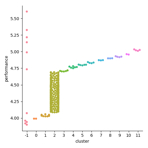
As we can see from above, this model configuration results identifies 13 packs in a 340 person race, with a number of runners not fitting within a pack at all (under the -1 label). We can modify this model to have a larger minimum pack size, or a larger/smaller distance between packs, which could be useful for other
But wait…we still have to supply a minimum distance between clusters, just like our home-grown clustering function. This difference is that unlike our homegrown function above, this model can handle any number of multiple dimensions and still compute the distance between clusters when clustering thousands or tens of thousands of data points.
Let’s move onto a more interesting example of clustering. Most athletes in track & field perform more than one event during track & field career. For example, most mid-distance runners have ran the 400m, 800m, and 1600m, and most long-distance runners have ran the 1600m, 3000m, and the 5000m. In some cases, there are long-distance runners who used to be mid-distance runners, and vice versa. To cluster events based on their performances in one event, we only have to cluster them based on their performances in one event. But to compare athletes who specialize in different events or who have skill in multiple events, we cannot always just compare their performances in one event, we have to compare their performances across all events. If we were to compare them across (n ) events, we would need to create vectors with ( n ) dimensions for each athlete.
\[\begin{pmatrix} 55m, 60m, 100m, 200m, ..., marathon \end{pmatrix}\]Using these vectors for each athlete we can calculate the Euclidean distance between each athlete to cluster the athletes. In this example, the euclidean distance is the sum of the combined differences in performances.
\[d(\bold{q},\bold{p}) = \sqrt{\sum^n_{\mathclap{i = 1}} (q_i - p_i)^2}\]But the range of times between the worlds record 55m time and a poor time is less than the difference between the world record 5000m time and a poor 5000m time. This would cause less elite sprinters to be clustered closer together than the less elite longer distance athletes, because the difference in times is greater. In fact, the longer the distance, the better the athlete would need to be in order to be closer to be considered close to another athlete. Since we are comparing athletes across disciplines, without bias, we will need to normalize our performances so that 55m performances are not clustered closer together than 5000m performances. In order to normalize our data, we need to scale our data so that they are all on the same scale, regardless of the performance. A common scale method is to ensure that all values are between 0 and 1. Since the distance between performances in each event is not the same, we will need to transform the performances of each event differently to ensure that the distance between performances in each event.
To do this, we will divide the performances of each athlete by the world record time in the event, using the men’s world record for male athletes, and the female world records for female athletes. If we really wanted to get detailed, we could use the world records for each age group, so that we could compare performances of masters/young athletes to the performances of prime athletes (in their 20s). But for now, we will use the overall world records for each gender.
\[d(\bold{q},\bold{p}, \bold{w}) = \sqrt{\sum^n_{\mathclap{i = 1}} ((q_i - p_i) / w_i)^2}\]The reason we are dividing by the world record is that we want times to be able to compare performances linearly across genders and events using the same units. By diving by the world record in the event, as your performances get worse, the result of the calculation gets larger linearly as your times get worse. This holds true for all running events, since the goal is to minimize the time needed to complete the race. If we were normalizing field event performances, we would want to divide the performance by the performance, as the goal is to get a larger distance/higher height, etc. This would preserve the linear growth of distance as performances get worse. You may also notice that depending on the demographic of the athletes, we may not need to use world record times, we could use NCAA Division I records for normalizing performances of NCAA Division I athletes, or Virginia High School League (VHSL) records for normalizing performances of Virginia High School athletes.
\[d(\bold{q},\bold{p}, \bold{w}) = \sqrt{\sum^n_{\mathclap{i = 1}} (w_i / (q_i - p_i))^2}\]It is worth noting that there are cases where a bias can be a good thing. For example, if we were clustering or comparing long-distance runners at long-distance runs we would not want sprinting events to have equal weight in the outcome, we would want the rankings to give greater weight to long-distance events. The same would go for sprinting, or middle-distance events. So there may be times where you may want to keep bias, or even introduce bias into your data/metrics to better achieve your objective.
Let’s get to preprocessing and clustering our athletes, but first we need to get our World Records to use for preprocessing from Wikipedia
{
	"50m": {
		"Indoor": {
			"male": 5.55,
			"female": 5.96
		}
	},
	"60m": {
		"Indoor": {
			"male": 6.34,
			"female": 6.92
		}
	},
	"100m": {
		"Outdoor": {
			"male": 9.58,
			"female": 10.49
		}
	},
	"200m": {
		"Outdoor": {
			"male": 19.19,
			"female": 21.34
		},
		"Indoor": {
			"male": 19.92,
			"female": 21.87
		}
	},
	"400m": {
		"Outdoor": {
			"male": 43.03,
			"female": 47.60
		},
		"Indoor": {
			"male": 44.52,
			"female": 49.59
		}
	},
	"800m": {
		"Outdoor": {
			"male": 100.91,
			"female": 113.28
		},
		"Indoor": {
			"male": 102.67,
			"female": 115.82
		}
	},
	"1000m": {
		"Outdoor": {
			"male": 131.96,
			"female": 148.98
		},
		"Indoor": {
			"male": 134.20,
			"female": 210.94
		}
	},
	"1500m": {
		"Outdoor": {
			"male": 206.00,
			"female": 230.07
		},
		"Indoor": {
			"male": 211.18,
			"female": 235.17
		}
	},
	"1 Mile": {
		"Outdoor": {
			"male": 323.13,
			"female": 252.56
		},
		"Indoor": {
			"male": 228.45,
			"female": 253.31
		}
	},
	"2000m": {
		"Outdoor": {
			"male": 284.79,
			"female": 323.75
		},
		"Indoor": {
			"female": 323.75
		}
	},
	"3000m": {
		"Outdoor": {
			"male": 440.79,
			"female": 486.11
		},
		"Indoor": {
			"male": 444.9,
			"female": 496.6
		}
	},
	"5000m": {
		"Outdoor": {
			"male": 757.35,
			"female": 851.15
		},
		"Indoor": {
			"male": 769.6,
			"female": 858.86
		}
	},
	"10000m": {
		"Outdoor": {
			"male": 1577.53,
			"female": 1757.45
		}
	},
	"20000m": {
		"Outdoor": {
			"male": 3385.98,
			"female": 3926.6
		}
	},
	"50m Hurdles": {
		"Indoor": {
			"male": 6.25,
			"female": 6.58
		}
	},
	"60m Hurdles": {
		"Indoor": {
			"male": 7.30,
			"female": 7.63
		}
	},
	"110m Hurdles": {
		"Outdoor": {
			"male": 12.8
		}
	},
	"100m Hurdles": {
		"Outdoor": {
			"female": 12.20
		}
	},
	"400m Hurdles": {
		"Outdoor": {
			"male": 46.78,
			"female": 52.34
		}
	},
	"3000m steeplechase": {
		"Outdoor": {
			"male": 473.63,
			"female": 524.32
		}
	},
	"High Jump": {
		"Outdoor": {
			"male": 2.45,
			"female": 2.09
		},
		"Indoor": {
			"male": 2.43,
			"female": 2.08
		}
	},
	"Long Jump": {
		"Outdoor": {
			"male": 8.95,
			"female": 7.52
		},
		"Indoor": {
			"male": 8.79,
			"female": 7.37
		}
	},
	"Triple Jump": {
		"Outdoor": {
			"male": 18.29,
			"female": 15.50
		},
		"Indoor": {
			"male": 17.92,
			"female": 15.36
		}
	},
	"Pole Vault": {
		"Outdoor": {
			"male": 6.16,
			"female": 5.06
		},
		"Indoor": {
			"male": 6.16,
			"female": 5.02
		}
	},
	"Shot Put": {
		"Outdoor": {
			"male": 23.12,
			"female": 22.63
		},
		"Indoor": {
			"male": 22.66,
			"female": 22.50
		}
	},
	"Discus Throw": {
		"Outdoor": {
			"male": 74.08,
			"female": 76.80
		}
	},
	"Hammer Throw": {
		"Outdoor": {
			"male": 86.74,
			"female": 82.98
		}
	},
	"Javelin Throw": {
		"Outdoor": {
			"male": 98.48,
			"female": 72.28
		}
	},
	"4 x 100m Relay": {
		"Outdoor": {
			"male": 36.84,
			"female": 40.82
		}
	},
	"4 x 200m Relay": {
		"Outdoor": {
			"male": 78.63,
			"female": 87.46
		},
		"Indoor": {
			"male": 82.11,
			"female": 92.41
		}
	},
	"4 x 400m Relay": {
		"Outdoor": {
			"male": 174.29,
			"female": 195.17
		},
		"Indoor": {
			"male": 181.39,
			"female": 203.37
		}
	},
	"4 x 800m Relay": {
		"Outdoor": {
			"male": 422.43,
			"female": 470.17
		},
		"Indoor": {
			"male": 431.3,
			"female": 485.89
		}
	},
	"Distance Medley Relay": {
		"Outdoor": {
			"male": 555.5,
			"female": 636.5
		}
	},
	"Sprint Medley Relay": {
		"Outdoor": {
			"male": 555.55,
			"female": 636.5
		}
	},
	"4 x 1500m relay": {
		"Outdoor": {
			"male": 862.22,
			"female": 993.58
		}
	}
}
In our example, we will just use KMeans to identify clusters. The reason for this is that, unlike our earlier example with race results from a single race, the density of PRs in events are dense when comparing a large number of athletes. Since density-based clustering use density changes in the data to determine where a cluster begins/ends, it would likely cluster the vast majority of athletes into a single cluster, which would not provide us with much useful information. KMeans uses a centroid-based clustering approach, which ignores the density of the data. The only downsides are that we must specify how many centroids (clusters) we wish to have, and that the clusters will tend to have roughly the same amount of points in each, which may or may be significant.
import pandas as pd


def preprocess(file_name, world_records, valid_events):
    world_records = world_records[world_records['event'].isin(valid_events)]
    world_records = world_records.set_index(['event', 'gender'])
    # only get the best fastest performance for each gender in each event, regardless of season
    world_records = world_records.groupby(['event', 'gender']).min()

    df = pd.read_csv(file_name)
    df = df[df['event'].isin(valid_events)]
    df = df.loc[df.groupby(['entity_id', 'event', 'gender'])['performance'].idxmin()]
    df = df.set_index(['event', 'gender']).join(world_records, rsuffix='_world')
    # normalize performances by world records by gender, ensuring the best performances are closest to 1.
    # to ensure the values are completely normalized, remove 1.0 so that performances are measured purely
    # by their distance from the world record
    df['normalized'] = df['performance'].divide(df['performance_world']) - 1.0
    df = df.pivot_table(index=['entity_id', 'gender'], columns='event', values='normalized')
    return df


if __name__ == '__main__':
    import time
    import json
    import seaborn
    from collections import Counter
    import matplotlib.pyplot as plt
    from sklearn import cluster, decomposition, pipeline, preprocessing

    performance_file_name = 'performances.csv.gz'
    world_records_file_name = 'world_records.json'
    with open(world_records_file_name, 'rb') as input_file:
        world_record_raw = json.load(input_file)

    # building a pandas DataFrame from the world_records data file
    world_records = dict(gender=[], event=[], performance=[])
    for event, event_data in world_record_raw.items():
        for season, season_data in event_data.items():
            for gender, value in season_data.items():
                world_records['gender'].append(gender.capitalize())
                #world_records['season'].append(season)
                world_records['performance'].append(value)
                world_records['event'].append(event)

    world_records = pd.DataFrame(world_records)
    valid_events = ['800M Run', '1000 Meters', '1500M Run', '3000 Meters', '5000M Run']
    print 'Preprocessing data'
    best_performances = preprocess(performance_file_name, world_records, valid_events)
    # only include athletes that have competed in all events being compared
    best_performances = best_performances[best_performances['800M Run'].notna() & best_performances['1000 Meters'].notna() & best_performances['1500M Run'].notna() & best_performances['3000 Meters'].notna() & best_performances['5000M Run'].notna()]
    print 'Preprocessed data'

    rows, columns = best_performances.shape
    performance_data = best_performances.as_matrix()

    transformer = decomposition.PCA(n_components=2)

    clf = pipeline.make_pipeline(
        preprocessing.StandardScaler(),
        cluster.KMeans()
    )

    print 'Clustering %s rows, and %s columns' % (rows, columns)
    start_time = time.time()
    predictions = clf.fit_predict(performance_data)
    cluster_counts = Counter(predictions)
    unique_clusters = set(predictions)
    duration = time.time() - start_time
    print 'Clustered %s rows, and %s columns into %s clusters in %s seconds' % (rows, columns, len(unique_clusters), duration)
    print 'Cluster Counts: %r' % cluster_counts.most_common(100)

    transformed_data = transformer.fit_transform(performance_data)
    df = pd.DataFrame(transformed_data)
    df['cluster'] = predictions

    best_performances['cluster'] = predictions

    seaborn.scatterplot(x=0, y=1, hue='cluster', legend='full', palette=seaborn.color_palette('hls', len(unique_clusters)), data=df)
    plt.show()

    transformer = decomposition.PCA(n_components=1)
    transformed_data = transformer.fit_transform(performance_data)
    df = pd.DataFrame(transformed_data)
    df['cluster'] = predictions

    seaborn.catplot(x='cluster', y=0, data=df)
    plt.show()
An8-core CPU needed only 0.7 seconds to cluster ~7000 athletes across 5 events. Let’s get a full view of the clusters of our ~7,000 athletes:
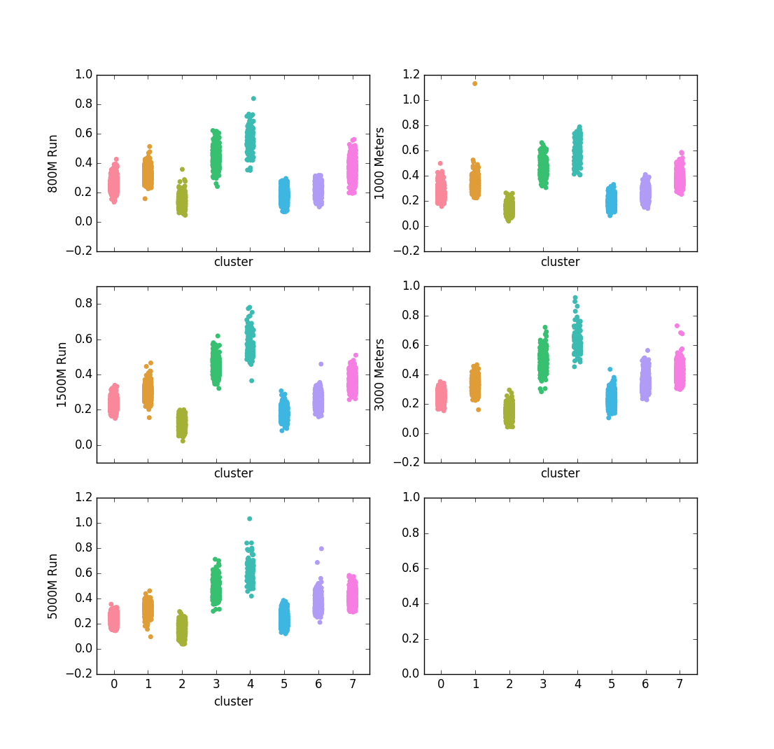
This chart shows how the athletes were clustered together, broken down by their PRs in these 5 events. Based on these results, Cluster #2 represents the fastest all-around distance athletes, while cluster #4 consists of the slowest all-around athletes. Based on the visual representation of these clusters, they are consistent in that faster athletes and slower athletes are consistently clustered into the same groups. This could be because there are high correlations between performances amongst these events.
print best_performances.corr()

event        1000 Meters  1500M Run  3000 Meters  5000M Run  800M Run
event
1000 Meters     1.000000   0.885239     0.827872   0.764290  0.878599
1500M Run       0.885239   1.000000     0.900009   0.857382  0.905061
3000 Meters     0.827872   0.900009     1.000000   0.913417  0.790621
5000M Run       0.764290   0.857382     0.913417   1.000000  0.725140
800M Run        0.878599   0.905061     0.790621   0.725140  1.000000
This correlation confirms our suspicions about why the data clusters seem to align with speed. Although, upon closer examination, the clusters do overlap in terms of the performances that are in each. The KMeans model clusters athletes based on all their PRs, equally weighted across all events we provided. So if an athlete has a fairly weak 1500m PR, but a superior 1000m, 3000m, and 5000m PR, then the model can determine that their overall superiority in events other than the 1500m, warrant them being being in a cluster with overall faster athletes. This is the strength of clustering athletes based on multiple events, we can cluster them based on a more holistic view of their abilities.
This approach could be also be used to cluster athletes based on their recent performances, which could be used by meet directors to put together more exciting/competitive competitions. The normalization technique could be used to compare athletes who ran during different eras (ex. Carl Lewis vs. Usain Bolt vs. Jesse Owens) to determine who had a better career. Or if we wanted to thoroughly compare the careers of athletes, we could add more dimensions, and evaluate athletes based on their average race, median race, best race, worst race, and using quartiles to provide a holistic view of their career, although normalizing the data would become more complicated (because we might have to normalize their performances based on what the world record was at the time of the competition).
While this clustering is interesting, it doesn’t tell us much about individual performances in a given competition. We would like some method for clustering individual performances based on attributes about those performances. We will call these attributes performance embeddings. For running performances, we can create performance embeddings using the individual splits of each athlete’s performance to group performances based on their individual splits. This allows us to group performances based on how similar all their splits are. A performance embedding for the hammer throw, may use the distances of each throwing attempt to represent the overall quality of their performance in that event at the competition. Today, we will be focusing on performance embeddings for the marathon.
First, we need to figure out how to represent our marathon performance embeddings using splits. We want each split, regardless of distance, to yield data in the same units. This ensures that splits over longer/shorter distances can be evaluated the same. We can normalize the splits by converting them to speed, or the pace of the athlete at that point in the race.
cumulative_performance_embeddings = []
for performance in performances:
    splits = performance.get('splits', [])
    performance_embedding = []
    for split in splits:
        normalized_split = split['cumulative_distance'] / split['cumulative_time']
        performance_embedding.append(normalized_split)
    cumulative_performance_embeddings.append(performance_embedding)
We also need to normalize our splits to only use the distance/time of that split since the previous split, not the cumulative distance/time in the competition. By only using the distance/time since the previous split, each dimension of our performance embedding depicts information for a specific segment of the competition. If we were to use the cumulative distances/times, splits taken from earlier in competition would be yield more information regarding the specific segment of the race, while splits taken later in the race would be biased based on the splits taken earlier in the race.
performances = []
for performance in performances:
    splits = performance.get('splits', [])
    previous_distance = 0.0
    previous_time = 0.0
    for split in splits:
        split_cumulative_distance = split['cumulative_distance']
        split_cumulative_time = split['cumulative_time']
        split['distance'] = split_cumulative_distance - previous_distance
        split['time'] = split_cumulative_time - previous_time
        previous_distance = split_cumulative_distance
        previous_time = split_cumulative_time

performance_embeddings = []
for performance in performances:
    splits = performance.get('splits', [])
    performance_embedding = []
    for split in splits:
        normalized_split = split['distance'] / split['time']
        performance_embedding.append(normalized_split)
    performance_embeddings.append(performance_embedding)
Now that we have our performance embeddings, we can begin clustering them. We will use AffinityPropogation clustering, as it can handle many clusters that may not be evenly sized. AffinityPropogation also returns results fairly quickly on race results from larger races, such as the New York City Marathon. DBSCAN can be effective for small races, where the field is fairly sparse, but I find that the epsilon value has to be carefully chosen based on the distance of the competition, and the range of talent of the competitors. But before we start clustering, let’s take a look at the embeddings:
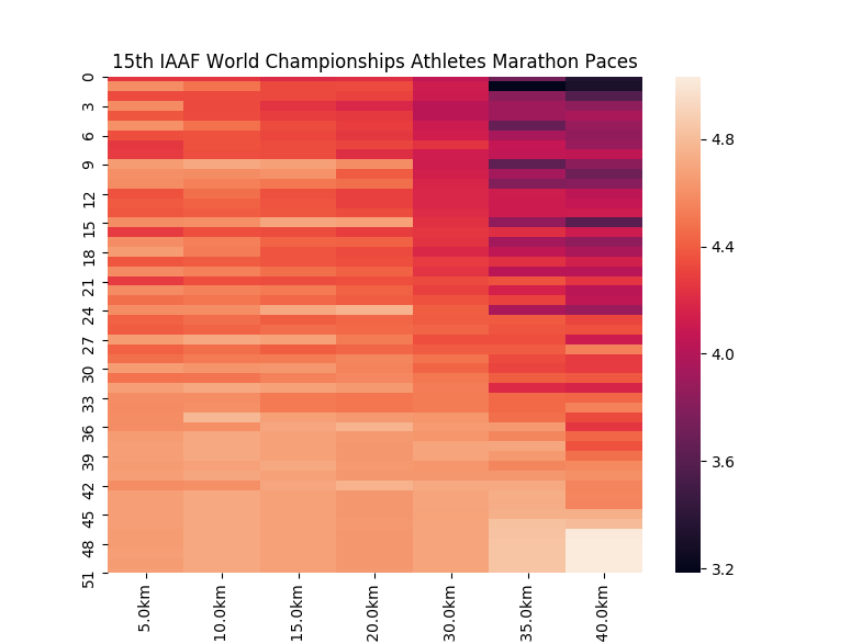
These embeddings are ordered where the 1st place finisher is at the top, and the last place finisher is at the bottom. We will use this same ordering in the other visualizations of these performances.
from sklearn.cluster import AffinityPropagation

clf = AffinityPropagation()
clusters = clf.fit_predict(performance_vectors)
Let’s visualize these clusters:
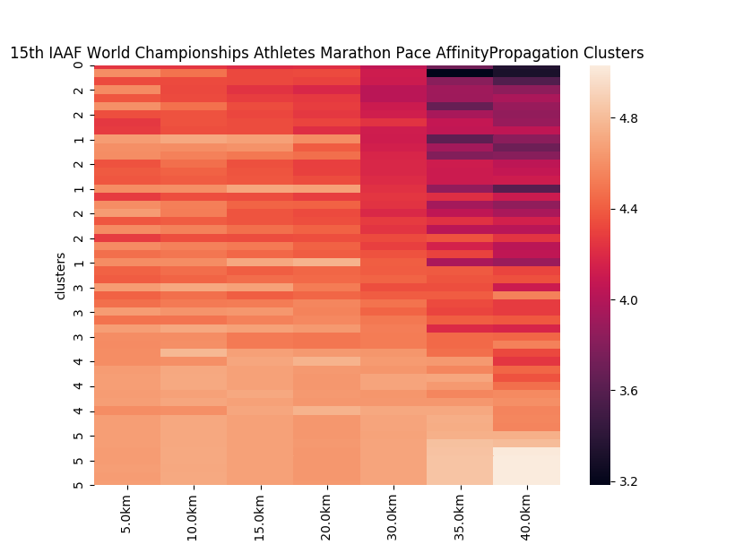
Let’s examine these clusters. Many of the cluster assignments are as one would expect: Performances with similar finish times tend to be clustered in the same groups, like in clusters 3, 4 and 5. But clusters 1 and 2 are mixed. Cluster #1, is made up of performances that started fast, slowed during the middle half of the competition and accelerated at the end of the race. Cluster #2 is made up of performances made up of negative splits (slow splits early in competition, and accelerate throughout the race). This method helps us group performances together based on the common trends in the splits.
You may be thinking that we could just use some simple functions to identify these patterns in performances. We could do that because the clusters are largely based on the patterns of split, but what if the runners followed patterns that we were not looking for? Or what if the runners all ran negative splits, but some runners increased pace at a different rate? We could write more code to handle these situations, but it would require writing code to handle every possible situation which would be time-consuming. These clustering algorithms are able to handle these situations without requiring writing additional code, which would allow us to handle any possible situation, across all competitions.
Lastly, you may have noticed that we did not touch cluster categorical data. We can measure the difference between a 17:32 5k split, and a 19:58 5k split (146 seconds), but how would you meaningfully calculate the distance between the pole vault, and the hammer throw? Or measure the difference between male and female? We need to use different methods for clustering categorical data ( source), and we need to use different methods for clustering data containing both categorical data and continuous data (source). Developers can use kmodes to cluster categorical data and mixed data. K-modes clustering is very similar to k-means clustering, except that the mode frequency of the categorical data fields is used to determine the placement of centroids rather than the mean of the continuous data fields.
Anomaly Detection🔗
Anomaly detection, in its broadest sense, is identifying items in our data that do not conform to the expected pattern. Using scikit-learn, we can train a model to detect anomalies in data. There are multiple types of anomaly detection, which differ mainly in how we define outliers in our data:
- Novelty detection -
The training data is not polluted by outliers, and we are interested in detecting anomalies in new observations.
- Outlier detection -
The training data contains outliers, and we need to fit the central mode of the training data, ignoring the deviant observations.
Based on these definitions and our running data, novelty detection should be used when we have a lot of good (non-anomalous) performances to train on, so the model will detect when a performance does not fit the dataset it was trained on. Outlier detection should be used when our training data may contain anomalies, and we want to identify those which are anomalies. Those performances that are anomalies can either been processed through a script to identify what makes them anomalies, or be flagged for a person to examine it themselves. So when could such a detector be useful?
- Does a performance break any world records? (novelty detection)
- Is a performance unusually slow/fast for a given distance? (outlier detection on performances for a given course)
- Is a performance unusually slow/fast for a given runner for a given distance? (novelty detection on performances by a given athlete)
- Did a runner run a race they do not usually run in a given season? (novelty detection on performances by a given athlete)
- Did a runner win/lose against a runner they normally do not run against? (novelty detection on performances from a set of races)
scikit-learn provides a OneClassSVM model for novelty detection. So this model would have some general applications for identifying fast/slow performances. The difficult part about training novelty detectors is ensuring we have good data. If we fit the model on our cleaned data (by excluding DNS and DNF performances) only performances that are not in our cleaned dataset will appear to be anomalies. This means that times that are faster than world records, or incredibly slow will appear to be anomalies. OneClassSVM would be would be very useful if trained on performances for individual athletes, any performances that differ from their existing performances could be flagged as an anomaly by the model, indicating that the athlete is injured, gotten faster, or in the worst case, may be using performance enhancing drugs.
to train our model, we will use pandas to remove any performances that are 0 (DNS) or extremely high (DNF) to ensure that such performances are identified as anomalies by our novelty detector.
import pandas as pd
from sklearn.svm import OneClassSVM
from sklearn.model_selection import train_test_split

df = pd.read_csv('track_field.csv')

# clean data of all times that are DNS (0) or DNF (999999) using my dataset
df = df[0 < df['time']< 999999]

data = data.values.tolist()

training_data, test_data = train_test_split(data, test_size=0.5)

# define and train our model based on training data
clf = OneClassSVM()
clf.fit(training_data)

# make predictions on our test_data that the model has not seen before
predictions = clf.predict(test_data)
# create separate arrays of normal performances and anomalies
normal = test_data[predictions == 1]
anomalies = test_data[predictions == -1]

print 'Normal: %r' % normal
print 'Normal Data Points: %r' % len(normal)

print 'Anomalies: %s' % anomalies
print 'Anomalous Data Points: %r' %  len(anomalies)
We just constructed a simple novelty detection model trained on half of all our performances. We can use the sklearn.covariance.EllipticEnvelope model for creating an outlier detection model, where we should not need to clean our data so rigorously or thoroughly. We will still remove our DNS/DNF performances to ensure that our model is not biased towads faster or slower performances.
import pandas as pd
from sklearn.covariance import EllipticEnvelope
from sklearn.model_selection import train_test_split

df = pd.read_csv('track_field.csv')

# clean data of all times that are DNS (0) or DNF (999999) using my dataset
df = df[0 < df['time']< 999999]

data = data.values.tolist()

training_data, test_data = train_test_split(data, test_size=0.5)

# define and train our model based on training data
clf = OneClassSVM()
clf.fit(training_data)

# make predictions on our test_data that the model has not seen before
predictions = clf.predict(test_data)

# create separate arrays of normal performances and anomalies
non_anomalies = test_data[predictions == 1]
anomalies = test_data[predictions == -1]

print 'Normal: %r' % non_anomalies
print 'Normal Data Points: %r' % len(non_anomalies)

print 'Anomalies: %s' % anomalies
print 'Anomalous Data Points: %r' %  len(anomalies)
The scikit-learn library offers a simple, effective starting point for deploying machine learning models that can provide useful information to runners and developers. While other libraries such as MXNet and Tensorflow provide methods for creating more advanced machine learning models, they require a more intimate knowledge of machine learning and the math behind them so we will save those for another post.
Biclustering🔗
One potential downside of clustering in many dimensions is that it can be difficult to explain how attributes contributed towards a row being assigned into a given cluster. Biclustering groups both the rows and columns of data in a matrix, which allows us to use column clusters to explain why a row was given a cluster assignment. You can recall that our embeddings above were formatted as a matrix as well, where rows were competitors, and columns were specific events. Biclustering assigns rows in a matrix to clusters, characterizing the clusters by mutually-exclusive clusters of columns. In the context of competitors being rows, and track & field events being columns, this would allow developers to both identify the cluster to which a competitor is assigned, and the cluster an event is assigned to.
Using these competitor and event clusters, developers can not only identify the cluster a competitor was assigned to, but determine why they were assigned to that particular cluster. Additionally, developers can determine if a competitor could have partial membership of another event cluster. If a competitor has performances in an event that are not common in their competitor cluster, that athlete’s event participation may exceed that of their cluster. In many cases, the athlete’s participation in other disciplines may minimal, but in other cases an athlete may be an outlier in that they regularly participate (and likely contribute to team successes) in events outside their primary discipline.
To have an example, we will use vectors of the number of times the person has participated in each event for clustering. The raw (unsorted) event is below:
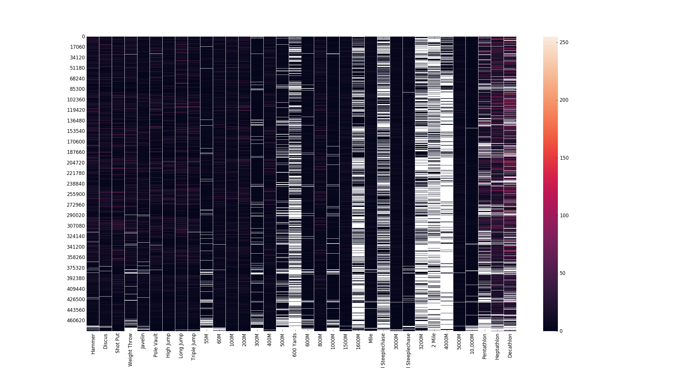
Our dataset contains entities who have competed in a wide range of events and scikit-learn’s biclustering implementation was able to cluster ~475,000 athletes based on their events in 8 seconds on an 8-core CPU. While the sklearn.clustering.biclustering.SpectralCoclustering model does not base its clusters on it’s neighbors , I sorted the columns (events) in my data matrix by discipline (throws, jumps, sprinting, long-distance running) and, for running events, in ascending order of the distance of the race. This does not have any impact on the output clusters, but does make the heatmap visualizing the data easier to read.
from sklearn.cluster.bicluster import SpectralCoclustering

import pandas as pd
import numpy as np
import matplotlib.pyplot as plt
import seaborn as sns

file_name = 'entity_event_participation.csv'
print 'processing %r' % file_name
df = pd.read_csv(file_name)

matrix = np.array(df.as_matrix())
# remove any athletes that have not participated in any events
matrix = matrix[~(matrix == 0).all(1)]

# remove any events which no athletes have competed in
zero_columns = np.argwhere(np.all(matrix[..., :] == 0, axis=0))
matrix = np.delete(matrix, zero_columns, axis=1)

# fit the model
model = SpectralCoclustering(n_clusters=6, random_state=0, n_jobs=-1).fit(matrix)

athlete_labels = model.row_labels_
event_labels = model.column_labels_

# sort athletes by their assigned label
fit_data = matrix[np.argsort(athlete_labels)]
fit_data = pd.DataFrame(fit_data, columns=df.columns)

# plot our results
#mask (do not render) blocks for events the athlete hasn't competed in
mask = fit_data == 0
sns.heatmap(fit_data, mask=mask)
plt.show()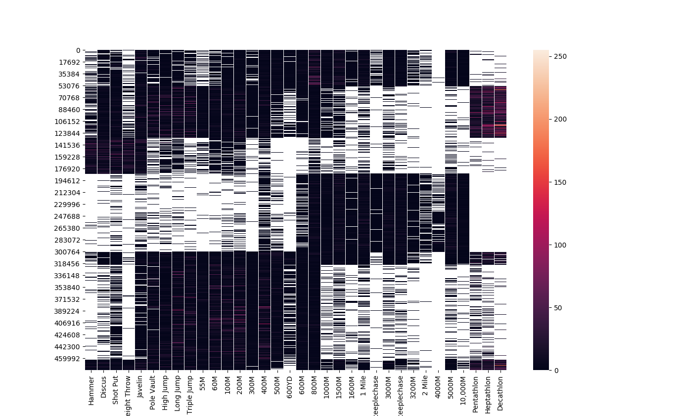
Based on our produced competitor clusters, the biclustering model clustered events into throwers, mid-distance and distances runners, sprinters, and two groups of multi-event competitors, one of which focuses on field events and sprint events, and another that participates in all types of events.
Performance Similarity🔗
A fundamental component of working with time series performances is being able to compare performances, and for that we need a distance measure. This could be useful for identifying athletes with similar racing styles, finding historical performances that match a given race strategy, or recommending training partners based on how they run races rather than just their finishing times.
A naive approach would use Euclidean distance between the split vectors of two performances. But that requires both performances to have the exact same number of splits taken at the exact same distances. In practice, splits are rarely so concistent. People choose different split distances, and chip timing/timing mats may not capture every athlete at every checkpoint. Additionally, athletes may speed up or slow down at different points in a race while still running fundamentally similar strategies.
Dynamic Time Warping (DTW) addresses these issues by finding the optimal alignment between two sequences, even when they differ in length (number of points) or are shifted in time. DTW was originally developed for speech recognition, but it has applications in any domain where we need to compare temporal sequences that may be warped or misaligned. Which is exactly what performance data is.
\[DTW(X, Y) = \min_{W} \sqrt{\sum_{(i,j) \in W} (x_i - y_j)^2}\]Where \( W \) is a warping path that aligns elements of sequence \( X \) to elements of sequence \( Y \).
Let’s consider a practical example of comparing the pacing strategies of two marathon runners. Runner A may have 5km splits, while Runner B has mile splits. Even if both runners ran negative splits (speeding up throughout the race), Euclidean distance would fail to capture this similarity because the split distances don’t align. DTW handles this by warping one sequence to align with the other, finding the minimum distance alignment.
from fastdtw import fastdtw
from scipy.spatial.distance import euclidean
import numpy as np

def normalize_splits(splits, distances):
    """
    Convert splits to pace (distance/time) for fair comparison
    across different split configurations.
    """
    paces = []
    prev_distance = 0.0
    prev_time = 0.0
    for split, distance in zip(splits, distances):
        segment_distance = distance - prev_distance
        segment_time = split - prev_time
        pace = segment_distance / segment_time  # speed in distance/time
        paces.append(pace)
        prev_distance = distance
        prev_time = split
    return paces

# Runner A: 5km splits (times in seconds)
runner_a_splits = [1080, 2175, 3285, 4410, 5550, 6705, 7875, 9060]  # ~18min/5km pace
runner_a_distances = [5, 10, 15, 20, 25, 30, 35, 40]  # km

# Runner B: mile splits (times in seconds)
runner_b_splits = [345, 696, 1053, 1416, 1785, 2160, 2541, 2928, 3321]  # ~5:45/mile pace
runner_b_distances = [1.609, 3.219, 4.828, 6.437, 8.047, 9.656, 11.265, 12.875, 14.484]  # km (miles converted)

# Normalize to paces for comparison
paces_a = normalize_splits(runner_a_splits, runner_a_distances)
paces_b = normalize_splits(runner_b_splits, runner_b_distances)

# Calculate DTW distance
distance, path = fastdtw(paces_a, paces_b, dist=euclidean)

print('DTW Distance: %.4f' % distance)
print('Alignment path: %s' % path)
The path variable contains tuples indicating which splits from each runner were aligned together. This alignment can reveal aspects of racing strategies. Like if both runners had a strong finishing kick, the final splits would align even if one runner had more splits than the other.
We can extend this approach to find the most similar historical performances to a given race:
from fastdtw import fastdtw
from scipy.spatial.distance import euclidean

def find_similar_performances(target_paces, historical_performances, top_n=5):
    """
    Find the most similar historical performances to a target performance
    using Dynamic Time Warping.

    Args:
        target_paces (list): Normalized paces of the target performance
        historical_performances (list): List of dicts with 'id', 'athlete', and 'paces'
        top_n (int): Number of similar performances to return

    Returns:
        list: Top N most similar performances with their DTW distances
    """
    similarities = []
    for performance in historical_performances:
        distance, path = fastdtw(target_paces, performance['paces'], dist=euclidean)
        similarities.append({
            'id': performance['id'],
            'athlete': performance['athlete'],
            'distance': distance,
            'alignment': path
        })

    # Sort by DTW distance (lower is more similar)
    similarities.sort(key=lambda x: x['distance'])
    return similarities[:top_n]

# Example usage with marathon performances
historical = [
    {'id': 1, 'athlete': 'Athlete A', 'paces': [4.62, 4.65, 4.68, 4.71, 4.75]},
    {'id': 2, 'athlete': 'Athlete B', 'paces': [4.80, 4.75, 4.70, 4.65, 4.60]},  # negative split
    {'id': 3, 'athlete': 'Athlete C', 'paces': [4.70, 4.70, 4.70, 4.70, 4.70]},  # even split
    {'id': 4, 'athlete': 'Athlete D', 'paces': [4.55, 4.60, 4.75, 4.85, 4.95]},  # positive split (fading)
]

# Find performances similar to a target negative split race
target = [4.78, 4.73, 4.68, 4.63, 4.58]
similar = find_similar_performances(target, historical, top_n=3)

for perf in similar:
    print('%s: DTW Distance = %.4f' % (perf['athlete'], perf['distance']))
This technique has practical applications for race analysis:
- Finding similar strategies: Find performances using similar pacing strategies (regardless of overall finishing time)
- Find similar athletes: Match athletes who run routinely have race patterns, which could indicate compatible training styles
- Predict performances: If an athlete’s early splits match an existing pattern, predict how the rest of the race might unfold
- Anomaly detection: Identify races where an athlete deviated significantly from their typical pattern
The standard DTW algorithm has \( O(nm) \) time complexity where \( n \) and \( m \) are the lengths of the two sequences. So adding another split to one of the performances used in the DTW calculated makes the calculation slowe For comparing a single performance against a large database of historical performances, this can become expensive. The fastdtw library implements an approximation algorithm that reduces complexity to \( O(n) \) while maintaining accuracy for most applications. But for our use case, even the \( O(nm) \) implementation would be feasible in production.
import time
from fastdtw import fastdtw
from scipy.spatial.distance import euclidean

# Benchmark DTW on larger sequences
large_sequence_a = [4.5 + (i * 0.01) for i in range(100)]  # 100 splits
large_sequence_b = [4.6 + (i * 0.008) for i in range(120)]  # 120 splits

start_time = time.time()
distance, path = fastdtw(large_sequence_a, large_sequence_b, dist=euclidean)
duration = time.time() - start_time

print('DTW Distance: %.4f' % distance)
print('Computation time: %.4f ms' % (duration * 1000))
print('Alignment path length: %d' % len(path))
DTW can also be combined with the clustering techniques I talked about earlier. Instead of using Euclidean distance as the metric for clustering performance embeddings, we can use DTW distance to cluster performances that have similar temporal patterns regardless of their exact split configurations. This would allow us to cluster marathon performances from different races with different checkpoint configurations, providing a more robust clustering across heterogeneous data sources.
Conclusion🔗
Machine learning has applications within sports, and has a low barrier to entry. Gathering data about a sport can enable insights to be gathered and acted upon considerably faster than by a human. This can free up humans to take on problems that are less defined that are critical for athlete’s performance and for spectator entertainment.